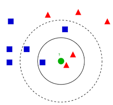
● K 최근접 이웃(K Nearest Neighnor, KNN)
- 특별한 예측 모델 없이 가장 가까운 데이터 포인트를 기반으로 예측 수행
- 분류와 회귀 모두 지원
- 필요한 라이브러리 import
import pandas as pd
import numpy as np
import multiprocessing
import matplotlib.pyplot as plt
plt.style.use(['seaborn-whitegrid'])

from sklearn.neighbors import KNeighborsClassifier, KNeighborsRegressor

# 시각화용
from sklearn.manifold import TSNE
# 사용할 예제 데이터세트
from sklearn.datasets import load_iris, load_breast_cancer, load_diabetes, fetch_california_housing

from sklearn.model_selection import train_test_split, cross_validate, GridSearchCV
from sklearn.preprocessing import StandardScaler
from sklearn.pipeline import make_pipeline
1. K 최근접 이웃(분류)
- 입력 데이터 포인트와 가장 가까운 k개의 훈련 데이터 포인트가 출력
- k개의 데이터 포인트 중 가장 많은 클래스가 예측 결과로 도출됨
1) 붓꽃 데이터
# 데이터 불러오기
X, y = load_iris(return_X_y = True)

# 훈련 데이터와 검증 데이터로 분리
X_train, X_test, y_train, y_test = train_test_split(X, y, test_size = 0.2)

# 범위 스케일링
scaler = StandardScaler()
X_train_scale = scaler.fit_transform(X_train)
X_test_scale = scaler.transform(X_test)

# K 최근접 이웃 모델 생성 후 학습(스케일링 하지 않은 모델로 학습)
model = KNeighborsClassifier()
model.fit(X_train, y_train)

print("학습 데이터 점수: {}".format(model.score(X_train, y_train)))
print("평가 데이터 점수: {}".format(model.score(X_test, y_test)))

# 출력 결과
학습 데이터 점수: 0.9666666666666667
평가 데이터 점수: 1.0


# K 최근접 이웃 모델 생성 후 학습(스케일링 한 모델로 학습)
model = KNeighborsClassifier()
model.fit(X_train_scaled, y_train)

print("학습 데이터 점수: {}".format(model.score(X_train_scaled, y_train)))
print("평가 데이터 점수: {}".format(model.score(X_test_scaled, y_test)))

# 출력 결과
학습 데이터 점수: 0.95
평가 데이터 점수: 1.0
- 교차검증으로 검증해주기
cross_validate(
    estimator = KNeighborsClassifier(),
    X = X, y = y,
    cv = 5,
    # cpu 코어 개수만큼 실행
    n_jobs = multiprocessing.cpu_count(),
    # 설명 출력
    verbose = True
)

# 출력 결과
[Parallel(n_jobs=8)]: Using backend LokyBackend with 8 concurrent workers.
[Parallel(n_jobs=8)]: Done   2 out of   5 | elapsed:    1.6s remaining:    2.5s
[Parallel(n_jobs=8)]: Done   5 out of   5 | elapsed:    1.7s finished
{'fit_time': array([0.00099683, 0.0009973 , 0.00099683, 0.00099564, 0.        ]),
 'score_time': array([0.00298977, 0.00199294, 0.00298977, 0.00299048, 0.00099659]),
 'test_score': array([0.96666667, 1.        , 0.93333333, 0.96666667, 1.        ])}
- 최적화(하이퍼 파라미터 조정)
param_grid = [{'n_neighbors': [3, 5, 7], # 이웃 생성 개수
               'weights': ['uniform', 'distance'], # 가중치 주는 방식(빈번하게 쓰는 건 distance)
               'algorithm': ['ball_tree', 'kd_tree', 'brute']}]

# 그리드 서치 옵션 설정
gs = GridSearchCV(
    estimator = KNeighborsClassifier(),
    param_grid = param_grid,
    n_jobs = multiprocessing.cpu_count(),
    verbose = True
)

gs.fit(X, y)
gs.best_estimator_
print('GridSearchCV best score: {}'.format(gs.best_score_))

# 출력 결과
GridSearchCV best score: 0.9800000000000001
# 위의 파라미터가 적용되었을 때 나온 최고의 점수는 약 0.98
- 시각화
# 격자 만드는 함수
def make_meshgrid(x, y, h = 0.02):
    x_min, x_max = x.min()-1, x.max()+1
    y_min, y_max = y.min()-1, y.max()+1
    xx, yy = np.meshgrid(np.arange(x_min, x_max, h),
                         np.arange(y_min, y_max, h))

    return xx, yy

# 격자 형태의 데이터를 예측 모델에 넣어서 각 격자점의 예측값을 구하고 나중에 예측값 별로 색깔 다르게 해서 해당 값의 범위 시각화
def plot_contours(clf, xx, yy, **params):
    Z = clf.predict(np.c_[xx.ravel(), yy.ravel()])
    Z = Z.reshape(xx.shape)
    out = plt.contourf(xx, yy, Z, **params)

    return out

# 요소를 두 개로 만들어 저차원으로 변환
tsne = TSNE(n_components = 2)
X_comp = tsne.fit_transform(X)

iris_comp_df = pd.DataFrame(data = X_comp)
iris_comp_df['Target'] = y
iris_comp_df
plt.scatter(X_comp[:, 0], X_comp[:, 1],
            c = y, cmap = plt.cm.coolwarm, s = 20, edgecolors = 'k')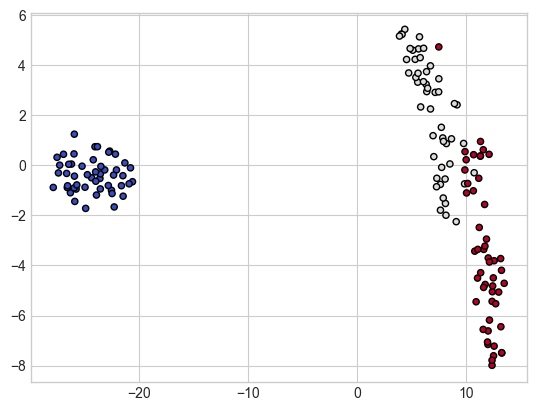
model = KNeighborsClassifier()
model.fit(X_comp, y)
predict = model.predict(X_comp)

xx, yy = make_meshgrid(X_comp[:, 0], X_comp[:, 1])
plot_contours(model, xx, yy, cmap = plt.cm.coolwarm, alpha = 0.8)
plt.scatter(X_comp[:, 0], X_comp[:, 1], c = y, cmap = plt.cm.coolwarm, s = 20, edgecolors = 'k')
- 각 데이터의 위치가 색깔 영역 내에 있으면 해당 색깔로 분류됨
2) 유방암 데이터
cancer = load_breast_cancer()
X, y = cancer.data, cancer.target
X_train, X_test, y_train, y_test = train_test_split(X, y, test_size = 0.2)


# 스케일링 하지 않은 데이터에 대한 예측 결과
model = KNeighborsClassifier()
model.fit(X_train, y_train)

print("학습 데이터 점수: {}".format(model.score(X_train, y_train)))
print("평가 데이터 점수: {}".format(model.score(X_test, y_test)))

# 출력 결과
학습 데이터 점수: 0.9472527472527472
평가 데이터 점수: 0.8947368421052632


# 스케일링 한 데이터에 대한 예측 결과
scaler = StandardScaler()
X_train_scale = scaler.fit_transform(X_train)
X_test_scale = scaler.transform(X_test)

model = KNeighborsClassifier()
model.fit(X_train_scale, y_train)

print("학습 데이터 점수: {}".format(model.score(X_train_scale, y_train)))
print("평가 데이터 점수: {}".format(model.score(X_test_scale, y_test)))

# 출력 결과
학습 데이터 점수: 0.9788732394366197
평가 데이터 점수: 1.0
- 교차 검증
estimator = make_pipeline(
    StandardScaler(),
    KNeighborsClassifier()
)
cross_validate(
    estimator = estimator,
    X = X, y = y,
    cv = 5,
    n_jobs = multiprocessing.cpu_count(),
    verbose = True
)

# 출력 결과
[Parallel(n_jobs=8)]: Using backend LokyBackend with 8 concurrent workers.
[Parallel(n_jobs=8)]: Done   2 out of   5 | elapsed:    1.8s remaining:    2.7s
[Parallel(n_jobs=8)]: Done   5 out of   5 | elapsed:    1.8s finished
{'fit_time': array([0.00199199, 0.0019908 , 0.00398612, 0.00299215, 0.00299025]),
 'score_time': array([0.06777287, 0.07774591, 0.07076406, 0.07574391, 0.06578112]),
 'test_score': array([0.96491228, 0.95614035, 0.98245614, 0.95614035, 0.96460177])}
# 점수가 0.96, 0.95 등으로 잘 나옴
- GridSearch
pipe = Pipeline(
    [('scaler', StandardScaler()),
     ('model', KNeighborsClassifier())]
)
param_grid = [{'model__n_neighbors': [3, 5, 7],
               'model__weights': ['uniform', 'distance'],
               'model__algorithm': ['ball_tree', 'kd_tree', 'brute']}]

gs = GridSearchCV(
    estimator = pipe,
    param_grid = param_grid,
    n_jobs = multiprocessing.cpu_count(),
    verbose = True
)
gs.fit(X, y)
gs.best_estimator_

# 출력 결과
KNeighborsClassifier(algorithm='ball_tree', n_neighbors=7)

print('GridSearchCV best score: {}'.format(gs.best_score_))

# 출력 결과
GridSearchCV best score: 0.9701288619779538
- 시각화
# 시각화를 위해 tsne를 이용해서 차원 축소(2차원으로)
tsne = TSNE(n_components = 2)
X_comp = tsne.fit_transform(X)

cacer_comp_df = pd.DataFrame(data= X_comp)
cancer_comp_df['Target'] = y
cancer_comp_df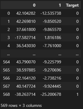
# 위의 표에서 0열과 1열을 각각 X좌표, y좌표로 하여 산점도 작성
plt.scatter(X_comp[:, 0], X_comp[:, 1], c = y, cmap = plt.cm.coolwarm, s = 20, edgecolor = 'k')
# 격자 만들어서 각 클래스별 영역 색깔로 구분하기
model = KNeighborsClassifier()
model.fit(X_comp, y)
predict = model.predict(X_comp)
xx, yy = make_meshgrid(X_comp[:, 0], X_comp[:, 1])
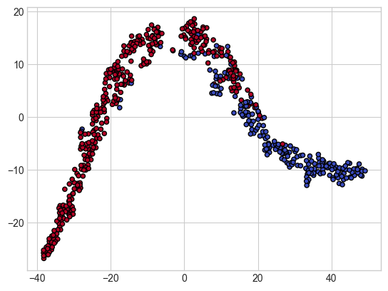
plot_contours(model, xx, yy, cmap = plt.cm.coolwarm, alpha = 0.8)
plt.scatter(X_comp[:, 0], X_comp[:, 1], c = y, cmap = plt.cm.coolwarm, s = 20, edgecolor = 'k')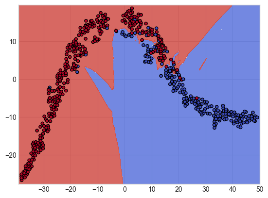
3) 와인 데이터
from sklearn.datasets import load_wine
wine = load_wine()
X, y = wine.data, wine.target
X_train, X_test, y_train, y_test = train_test_split(X, y, test_size = 0.2)

model = KNeighborsClassifier()
model.fit(X_train, y_train)

print("학습 데이터 점수: {}".format(model.score(X_train, y_train)))
print("평가 데이터 점수: {}".format(model.score(X_test, y_test)))

# 출력 결과
학습 데이터 점수: 0.7887323943661971
평가 데이터 점수: 0.6111111111111112


scaler = StandardScaler()
X_train_scale = scaler.fit_transform(X_train)
X_test_scale = scaler.transform(X_test)

model = KNeighborsClassifier()
model.fit(X_train_scale, y_train)

print("학습 데이터 점수: {}".format(model.score(X_train_scale, y_train)))
print("평가 데이터 점수: {}".format(model.score(X_test_scale, y_test)))

# 출력 결과
학습 데이터 점수: 0.9859154929577465
평가 데이터 점수: 0.9444444444444444
# 교차검증
estimator = make_pipeline(
StandardScaler(),
KNeighborsClassifier()
)
cross_validate(
estimator = estimator,
X = X, y = y,
cv = 5,
n_jobs = multiprocessing.cpu_count(),
verbose = True
)
# 출력 결과
[Parallel(n_jobs=8)]: Using backend LokyBackend with 8 concurrent workers.
[Parallel(n_jobs=8)]: Done 2 out of 5 | elapsed: 1.7s remaining: 2.5s
[Parallel(n_jobs=8)]: Done 5 out of 5 | elapsed: 1.7s finished
{'fit_time': array([0.00299406, 0.00099683, 0.00199389, 0.00199318, 0.00198913]),
'score_time': array([0.00398278, 0.00199437, 0.00199485, 0.00199366, 0.00199366]),
'test_score': array([0.94444444, 0.94444444, 0.97222222, 1. , 0.88571429])}# GridSearch
pipe = Pipeline(
[('scaler', StandardScaler()),
('model', KNeighborsClassifier())]
)
param_grid = [{'model__n_neighbors': [3, 5, 7],
'model__weights': ['uniform', 'distance'],
'model__algorithm': ['ball_tree', 'kd_tree', 'brute']}]
gs = GridSearchCV(
estimator = pipe,
param_grid = param_grid,
n_jobs = multiprocessing.cpu_count(),
verbose = True
)
gs.fit(X, y)
gs.best_estimator_
# 출력 결과
KNeighborsClassifier(algorithm='ball_tree', n_neighbors=7
print('GridSearchCV best score: {}'.format(gs.best_score_))
# 출력 결과
GridSearchCV best score: 0.9665079365079364# 시각화
tsne = TSNE(n_components = 2)
X_comp = tsne.fit_transform(X)
wine_comp_df = pd.DataFrame(data= X_comp)
wine_comp_df['Target'] = y
wine_comp_df
# 시각화
plt.scatter(X_comp[:, 0], X_comp[:, 1], c = y, cmap = plt.cm.coolwarm, s = 20, edgecolor = 'k')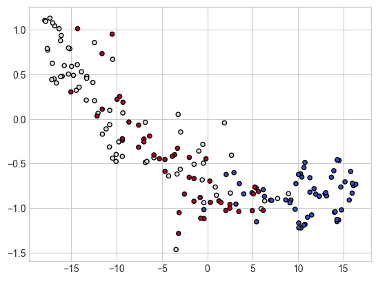
# 시각화
model = KNeighborsClassifier()
model.fit(X_comp, y)
predict = model.predict(X_comp)

xx, yy = make_meshgrid(X_comp[:, 0], X_comp[:, 1])
plot_contours(model, xx, yy, cmap = plt.cm.coolwarm, alpha = 0.8)
plt.scatter(X_comp[:, 0], X_comp[:, 1], c = y, cmap = plt.cm.coolwarm, s = 20, edgecolor = 'k')
2. K 최근접 이웃(회귀)
- k 최근접 이웃 분류와 마찬가지로 예측에 이웃 데이터 포인트 사용
- 이웃 데이터 포인트의 평균이 예측 결과
1) 당뇨병 데이터
diabetes = load_diabetes()
X, y = diabetes.data, diabetes.target
X_train, X_test, y_train, y_test =train_test_split(X, y, test_size = 0.2)

# 스케일링 하기 전
mdoel = KNeighborsRegressor()
model.fit(X_train, y_train)
print("학습 데이터 점수: {}".format(model.score(X_train, y_train)))
print("평가 데이터 점수: {}".format(model.score(X_test, y_test)))

# 출력 결과
학습 데이터 점수: 0.16997167138810199
평가 데이터 점수: 0.0


# 스케일링 한 후
scaler = StandardScaler()
X_train_scale = scaler.fit_transform(X_train)
X_test_scale = scaler.transform(X_test)

model.fit(X_train_scale, y_train)
print("학습 데이터 점수: {}".format(model.score(X_train_scale, y_train)))
print("평가 데이터 점수: {}".format(model.score(X_test_scale, y_test)))

# 출력 결과
학습 데이터 점수: 0.17280453257790368
평가 데이터 점수: 0.0
- 교차 검증
estimator = make_pipeline(
    StandardScaler(),
    KNeighborsRegressor()
)
cross_validate(
    estimator = estimator,
    X = X, y = y,
    cv = 5,
    n_jobs = multiprocessing.cpu_count(),
    verbose = True
)

# 출력 결과
[Parallel(n_jobs=8)]: Using backend LokyBackend with 8 concurrent workers.
[Parallel(n_jobs=8)]: Done   2 out of   5 | elapsed:    1.9s remaining:    2.9s
[Parallel(n_jobs=8)]: Done   5 out of   5 | elapsed:    1.9s finished
{'fit_time': array([0.00099659, 0.00099659, 0.00099659, 0.00190091, 0.00199246]),
 'score_time': array([0.00099754, 0.00099754, 0.00099754, 0.00199389, 0.00199389]),
 'test_score': array([0.32911328, 0.37917455, 0.42454147, 0.30674261, 0.40528841])}
- GridSearch
pipe = Pipeline(
    [('scaler', StandardScaler()),
     ('model', KNeighborsRegressor())]
)
param_grid = [{'model__n_neighbors': [3, 5, 7],
               'model__weights': ['uniform', 'distance'],
               'model__algorithm': ['ball_tree', 'kd_tree', 'brute']}]
gs = GridSearchCV(
    estimator = pipe,
    param_grid = param_grid,
    n_jobs = multiprocessing.cpu_count(),
    verbose = True
)
gs.fit(X, y)

gs.best_estimator_

# 출력 결과
KNeighborsRegressor(algorithm='ball_tree', n_neighbors=7, weights='distance')

print('GridSearchCV best score: {}'.format(gs.best_score_))

# 출력 결과
GridSearchCV best score: 0.40751067010691555
- 시각화
tsne = TSNE(n_components = 1) # 회귀이므로 클래스 구분이 없으니까 차원을 한 개로
X_comp = tsne.fit_transform(X)

diabetes_comp_df = pd.DataFrame(data = X_comp)
diabetes_comp_df['target'] = y
diabetes_comp_df
plt.scatter(X_comp, y, c = 'b', cmap = plt.cm.coolwarm, s = 20, edgecolor = 'k')
model = KNeighborsRegressor()
model.fit(X_comp, y)
predict = model.predict(X_comp)

# 실제 데이터
plt.scatter(X_comp, y, c = 'b', cmap = plt.cm.coolwarm, s = 20, edgecolor = 'k')
# 예측한 데이터
plt.scatter(X_comp, predict, c = 'r', cmap = plt.cm.coolwarm, s = 20, edgecolor = 'k')
2) 캘리포니아 주택 가격 데이터
california = fetch_california_housing()
X, y = california.data, california.target
X_train, X_test, y_train, y_test =train_test_split(X, y, test_size = 0.2)

# 스케일링 하기 전
mdoel = KNeighborsRegressor()
model.fit(X_train, y_train)
print("학습 데이터 점수: {}".format(model.score(X_train, y_train)))
print("평가 데이터 점수: {}".format(model.score(X_test, y_test)))

# 출력 결과
학습 데이터 점수: 0.44567719080525625
평가 데이터 점수: 0.16779095299754077


# 스케일링 한 후
scaler = StandardScaler()
X_train_scale = scaler.fit_transform(X_train)
X_test_scale = scaler.transform(X_test)

model.fit(X_train_scale, y_train)
print("학습 데이터 점수: {}".format(model.score(X_train_scale, y_train)))
print("평가 데이터 점수: {}".format(model.score(X_test_scale, y_test)))

# 출력 결과
학습 데이터 점수: 0.7908165274051309
평가 데이터 점수: 0.7034387252032074
estimator = make_pipeline(
StandardScaler(),
KNeighborsRegressor()
)
cross_validate(
estimator = estimator,
X = X, y = y,
cv = 5,
n_jobs = multiprocessing.cpu_count(),
verbose = True
)
# 출력 결과
[Parallel(n_jobs=8)]: Using backend LokyBackend with 8 concurrent workers.
[Parallel(n_jobs=8)]: Done 2 out of 5 | elapsed: 2.2s remaining: 3.3s
[Parallel(n_jobs=8)]: Done 5 out of 5 | elapsed: 2.3s finished
{'fit_time': array([0.06188369, 0.06133103, 0.06877017, 0.05989504, 0.05780768]),
'score_time': array([0.44215131, 0.38237071, 0.38546276, 0.4753325 , 0.43939376]),
'test_score': array([0.47879396, 0.4760079 , 0.57624554, 0.50259828, 0.57228584])}pipe = Pipeline(
[('scaler', StandardScaler()),
('model', KNeighborsRegressor())]
)
param_grid = [{'model__n_neighbors': [3, 5, 7],
'model__weights': ['uniform', 'distance'],
'model__algorithm': ['ball_tree', 'kd_tree', 'brute']}]
gs = GridSearchCV(
estimator = pipe,
param_grid = param_grid,
n_jobs = multiprocessing.cpu_count(),
verbose = True
)
gs.fit(X, y)
gs.best_estimator_
# 출력 결과
KNeighborsRegressor(algorithm='ball_tree', n_neighbors=7, weights='distance')
print('GridSearchCV best score: {}'.format(gs.best_score_))
# 출력 결과
GridSearchCV best score: 0.5376515274379832tsne = TSNE(n_components = 1) # 회귀이므로 클래스 구분이 없으니까 차원을 한 개로
X_comp = tsne.fit_transform(X)
diabetes_comp_df = pd.DataFrame(data = X_comp)
diabetes_comp_df['target'] = y
diabetes_comp_df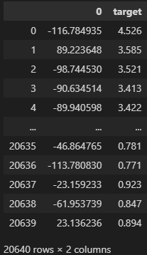
plt.scatter(X_comp, y, c = 'b', cmap = plt.cm.coolwarm, s = 20, edgecolor = 'k')
model = KNeighborsRegressor()
model.fit(X_comp, y)
predict = model.predict(X_comp)

# 실제 데이터
plt.scatter(X_comp, y, c = 'b', cmap = plt.cm.coolwarm, s = 20, edgecolor = 'k')
# 예측한 데이터
plt.scatter(X_comp, predict, c = 'r', cmap = plt.cm.coolwarm, s = 20, edgecolor = 'k')
'Python > Machine Learning' 카테고리의 다른 글
| [머신러닝 알고리즘] 서포트 벡터 머신 (0) | 2023.01.13 |
|---|---|
| [머신러닝 알고리즘] 나이브 베이즈 (0) | 2023.01.10 |
| [머신러닝 알고리즘] 로지스틱 회귀 (0) | 2023.01.04 |
| [머신러닝 알고리즘] 선형 회귀(2) (0) | 2023.01.02 |
| [머신러닝 알고리즘] 선형 회귀(1) (0) | 2022.12.29 |