● 결정 트리(Decision Tree)
- 분류와 회귀에 사용되는 지도 학습 방법
- 데이터 특성으로부터 추론된 결정 규칙을 통해 값을 예측
- if-then-else 결정 규칙을 통해 데이터 학습
- 트리의 깊이가 깊을 수록 복잡한 모델
- 결정 트리의 장점
- 이해와 해석이 쉬움
- 시각화 용이
- 많은 데이터 전처리 필요 x
- 수치형, 범주형 모두 다룰 수 있음
- ...
- 결정 트리에 필요한 라이브러리
# 필요 라이브러리
import pandas as pd
import numpy as np
import graphviz
import multiprocessing
import matplotlib.pyplot as plt
from sklearn.datasets import load_iris, load_wine, load_breast_cancer, load_diabetes
from sklearn import tree
from sklearn.tree import DecisionTreeClassifier, DecisionTreeRegressor
from sklearn.preprocessing import StandardScaler
from sklearn.model_selection import cross_val_score
from sklearn.pipeline import make_pipeline
1. 결정 트리를 활용한 분류(DecisionTreeClassifier())
- DecisionTreeClassifier는 분류를 위한 결정 트리 모델
- 두 개의 배열 X, y를 입력받음
- X는 [n_samples, n_features] 크기의 데이터 특성 배열
- y는 [n_samples] 크기의 정답 배열
X = [[0, 0], [1, 1]]
y = [0, 1]

# X가 [0, 0]일 때는 y가 0, X가 [1, 1]일 때는 y가 1 과 같이 분류
model = tree.DecisionTreeClassifier()
model = model.fit(X, y)

# X에 [2, 2]를 줬을 때 0과 1 중 어디로 분류될 지
model.predict([[2., 2.]])

# 출력 결과
array([1]) # 1로 분류됨


# X에 [2, 2]를 줬을 때 0과 1에 각각 분류될 확률
model.predict_proba([[2., 2.]])

# 출력 결과
array([[0., 1.]]) # 1이 선택될 확률이 100%로 나옴
1) 붓꽃 데이터 분류(전처리 x)
model = DecisionTreeClassifier()
cross_val_score(
    estimator = model,
    X = iris.data, y = iris.target,
    cv = 5,
    n_jobs = multiprocessing.cpu_count()
)

# 출력 결과
array([0.96666667, 0.96666667, 0.9       , 1.        , 1.        ])
2) 붓꽃 데이터 분류(전처리 o)
model = make_pipeline(
    StandardScaler(),
    DecisionTreeClassifier()
)

cross_val_score(
    estimator = model,
    X = iris.data, y = iris.target,
    cv = 5,
    n_jobs = multiprocessing.cpu_count()
)

# 출력 결과
array([0.96666667, 0.96666667, 0.9       , 1.        , 1.        ])
- 전처리 한 것과 하지 않은 것의 결과에 차이가 없는데, 결정 트리는 규칙을 학습하기 때문에 전처리에 큰 영향을 받지 않음
3) 학습된 결정 트리 시각화
- 텍스트 형태로 시각화
# 트리를 텍스트로 추출
r = tree.export_text(decision_tree = model, feature_names = iris.feature_names)
print(r)

# 출력 결과
|--- petal length (cm) <= 2.45
|   |--- class: 0
|--- petal length (cm) >  2.45
|   |--- petal width (cm) <= 1.75
|   |   |--- petal length (cm) <= 4.95
|   |   |   |--- petal width (cm) <= 1.65
|   |   |   |   |--- class: 1
|   |   |   |--- petal width (cm) >  1.65
|   |   |   |   |--- class: 2
|   |   |--- petal length (cm) >  4.95
|   |   |   |--- petal width (cm) <= 1.55
|   |   |   |   |--- class: 2
|   |   |   |--- petal width (cm) >  1.55
|   |   |   |   |--- petal length (cm) <= 5.45
|   |   |   |   |   |--- class: 1
|   |   |   |   |--- petal length (cm) >  5.45
|   |   |   |   |   |--- class: 2
|   |--- petal width (cm) >  1.75
|   |   |--- petal length (cm) <= 4.85
|   |   |   |--- sepal width (cm) <= 3.10
|   |   |   |   |--- class: 2
|   |   |   |--- sepal width (cm) >  3.10
|   |   |   |   |--- class: 1
|   |   |--- petal length (cm) >  4.85
|   |   |   |--- class: 2
- plot 형태로 시각화
tree.plot_tree(model)
- graphviz 시각화
dot_data = tree.export_graphviz(decision_tree = model,
                                feature_names = iris.feature_names,
                                class_names = iris.target_names,
                                filled = True, rounded = True,
                                special_characters = True)
# filled는 상자에 색깔을 칠할 것인지
# rounded는 상자 모서리를 둥글게 할 것인지
# special_characters는 특수문자

graph = graphviz.Source(dot_data)
graph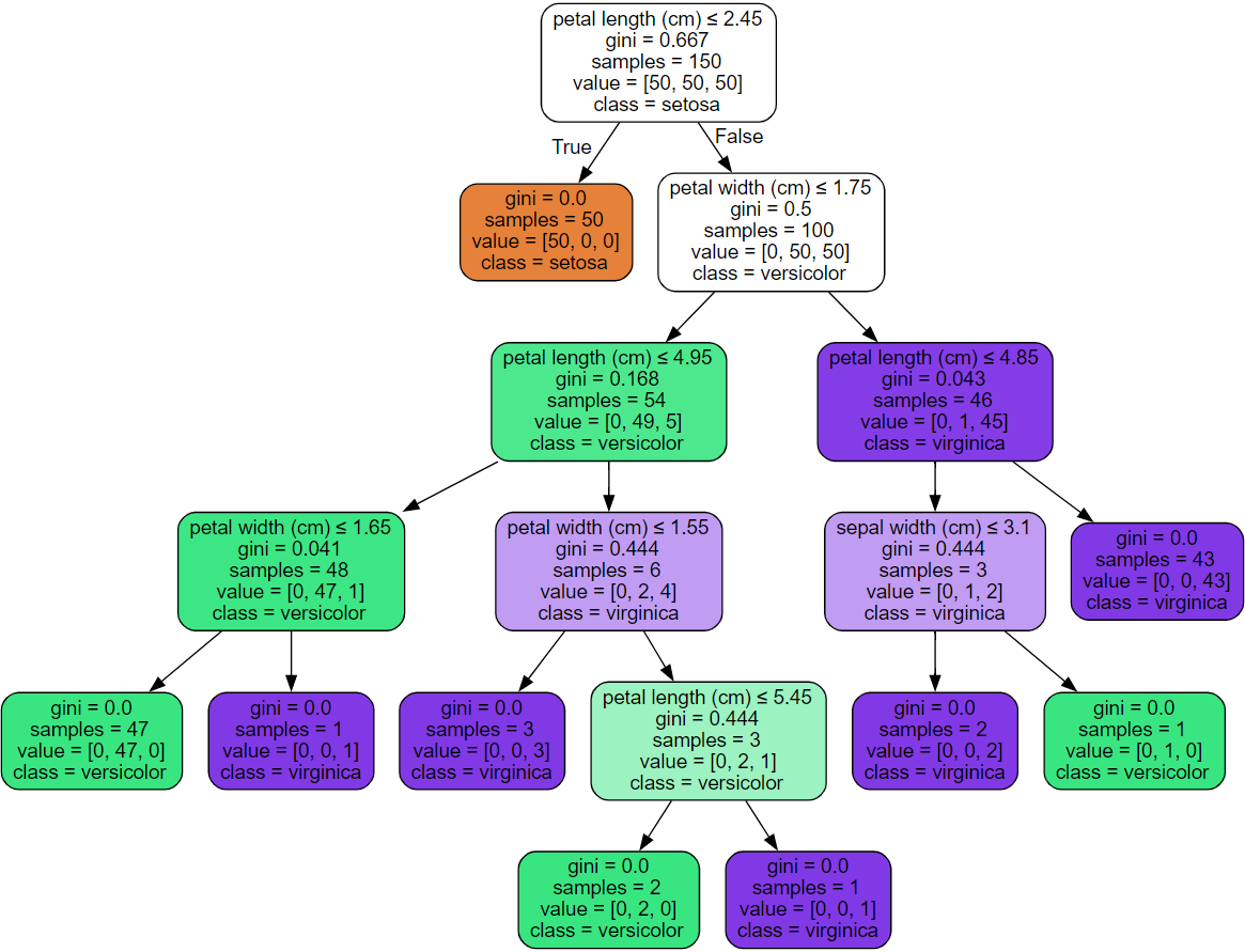
- 결정 경계 시각화
n_classes = 3
plot_colors = 'ryb'
plot_step = 0.02

# 결정경계 시각화
plt.figure(figsize = (16, 8))
# pairidx는 자동으로 1씩 늘어나는 숫자 변수
# pair는 그래프의 x축과 y축에 각각 [0번째 변수, 1번째 변수], [0번째 변수, 2번째 변수],...를 넣음을 의미
for pairidx, pair in enumerate([[0, 1], [0, 2], [0, 3], [1, 2], [1, 3], [2, 3]]):
    X = iris.data[:, pair]
    y = iris.target

    model = DecisionTreeClassifier()
    model = model.fit(X, y)

    # 그래프는 2행 3열의 형태로 배치
    plt.subplot(2, 3, pairidx + 1)

    # meshgrid로 각 분류 영역 색깔로 구분
    x_min, x_max = X[:, 0].min() - 1, X[:, 0].max() + 1
    y_min, y_max = X[:, 1].min() - 1, X[:, 1].max() + 1
    xx, yy = np.meshgrid(np.arange(x_min, x_max, plot_step),
                         np.arange(y_min, y_max, plot_step))
    plt.tight_layout(h_pad = 0.5, w_pad = 0.5, pad = 2.5)

    Z = model.predict(np.c_[xx.ravel(), yy.ravel()])
    Z = Z.reshape(xx.shape)
    cs = plt.contourf(xx, yy, Z, cmap = plt.cm.RdYlBu)

    plt.xlabel(iris.feature_names[pair[0]])
    plt.ylabel(iris.feature_names[pair[1]])

    # 전체 분류 개수(3개의 클래스)에 각각 plot_colors('r(red)y(yello)b(blue)')를 부여
    for i, color in zip(range(n_classes), plot_colors):
        idx = np.where(y == i)
        plt.scatter(X[idx, 0], X[idx, 1], c = color, label = iris.target_names[i],
                    cmap = plt.cm.RdYlBu, edgecolor = 'b', s = 15)

plt.suptitle("Decision surface")
plt.legend(loc = 'lower right', borderpad = 0, handletextpad = 0)
# loc: 범례의 위치는 오른쪽 아래
# borderpad: 범례 경계에 부분적인 빈 공간 입력
# handletextpad: 범례의 handle과 text 사이의 공간
plt.axis('tight')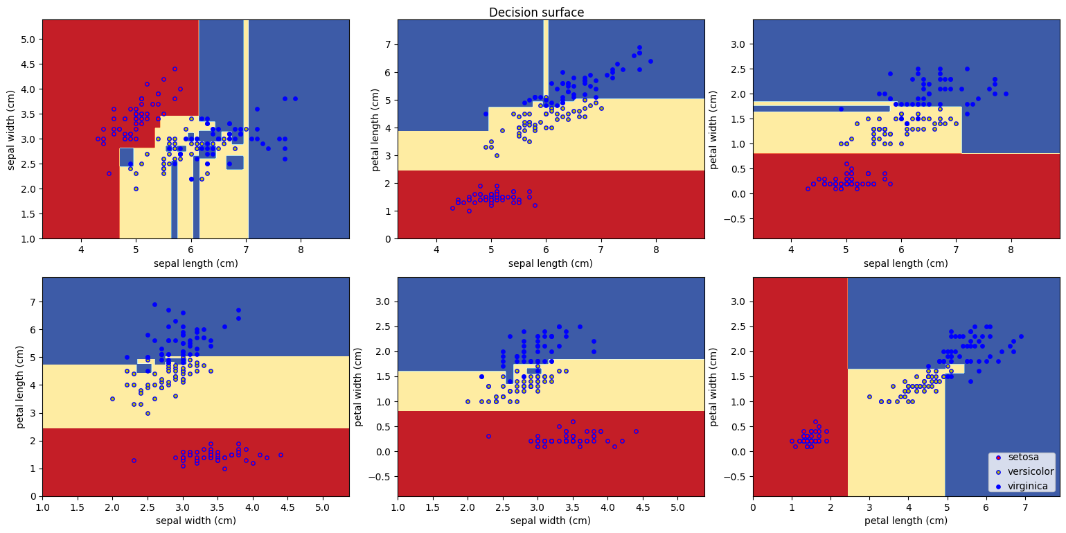
- max_depth를 2로 줬을 때

4) 와인 데이터 분류(전처리 x)
model = DecisionTreeClassifier()
cross_val_score(
    estimator = model,
    X = wine.data, y = wine.target,
    cv = 5,
    n_jobs = multiprocessing.cpu_count()
)

# 출력 결과
array([0.94444444, 0.86111111, 0.88888889, 0.91428571, 0.85714286])
5) 와인 데이터 분류(전처리 o)
model = make_pipeline(StandardScaler(), DecisionTreeClassifier())

cross_val_score(
    estimator = model,
    X = wine.data, y = wine.target,
    cv = 5,
    n_jobs = multiprocessing.cpu_count()
)

# 출력 결과
array([0.94444444, 0.80555556, 0.91666667, 0.91428571, 0.85714286])
6) 학습된 결정 트리 시각화
- 텍스트 형식으로 시각화
model = DecisionTreeClassifier()
model.fit(wine.data, wine.target)

r = tree.export_text(decision_tree = model, feature_names = wine.feature_names)
print(r)

# 출력 결과
|--- proline <= 755.00
|   |--- od280/od315_of_diluted_wines <= 2.11
|   |   |--- hue <= 0.94
|   |   |   |--- flavanoids <= 1.58
|   |   |   |   |--- class: 2
|   |   |   |--- flavanoids >  1.58
|   |   |   |   |--- class: 1
|   |   |--- hue >  0.94
|   |   |   |--- ash <= 2.45
|   |   |   |   |--- class: 1
|   |   |   |--- ash >  2.45
|   |   |   |   |--- class: 2
|   |--- od280/od315_of_diluted_wines >  2.11
|   |   |--- flavanoids <= 0.80
|   |   |   |--- class: 2
|   |   |--- flavanoids >  0.80
|   |   |   |--- alcohol <= 13.17
|   |   |   |   |--- class: 1
|   |   |   |--- alcohol >  13.17
|   |   |   |   |--- magnesium <= 98.50
|   |   |   |   |   |--- class: 1
|   |   |   |   |--- magnesium >  98.50
|   |   |   |   |   |--- class: 0
|--- proline >  755.00
|   |--- flavanoids <= 2.17
|   |   |--- hue <= 0.80
|   |   |   |--- class: 2
|   |   |--- hue >  0.80
|   |   |   |--- class: 1
|   |--- flavanoids >  2.17
|   |   |--- magnesium <= 135.50
|   |   |   |--- class: 0
|   |   |--- magnesium >  135.50
|   |   |   |--- class: 1
- plot 형태로 시각화
tree.plot_tree(model)
- graphviz로 시각화

- 결정 경계 시각화
n_classes = 3
plot_colors = 'ryb'
plot_step = 0.02

# 결정경계 시각화
plt.figure(figsize = (16, 8))
for pairidx, pair in enumerate([[0, 1], [0, 2], [0, 3], [1, 2], [1, 3], [2, 3]]):
    X = wine.data[:, pair]
    y = wine.target

    model = DecisionTreeClassifier()
    model = model.fit(X, y)

    plt.subplot(2, 3, pairidx + 1)

    x_min, x_max = X[:, 0].min() - 1, X[:, 0].max() + 1
    y_min, y_max = X[:, 1].min() - 1, X[:, 1].max() + 1
    xx, yy = np.meshgrid(np.arange(x_min, x_max, plot_step),
                         np.arange(y_min, y_max, plot_step))
    plt.tight_layout(h_pad = 0.5, w_pad = 0.5, pad = 2.5)

    Z = model.predict(np.c_[xx.ravel(), yy.ravel()])
    Z = Z.reshape(xx.shape)
    cs = plt.contourf(xx, yy, Z, cmap = plt.cm.RdYlBu)

    plt.xlabel(iris.feature_names[pair[0]])
    plt.ylabel(iris.feature_names[pair[1]])

    for i, color in zip(range(n_classes), plot_colors):
        idx = np.where(y == i)
        plt.scatter(X[idx, 0], X[idx, 1], c = color, label = iris.target_names[i],
                    cmap = plt.cm.RdYlBu, edgecolor = 'b', s = 15)

plt.suptitle("Decision surface")
plt.legend(loc = 'lower right', borderpad = 0, handletextpad = 0)
plt.axis('tight')

- max_depth를 2로 줬을 때

7) 유방암 데이터 분류(전처리 x)
model = DecisionTreeClassifier()
cross_val_score(
    estimator = model,
    X = cancer.data, y = cancer.target,
    cv = 5,
    n_jobs = multiprocessing.cpu_count()
)

# 출력 결과
array([0.9122807 , 0.90350877, 0.92982456, 0.93859649, 0.89380531])
8) 유방암 데이터 분류(전처리 o)
model = make_pipeline(StandardScaler(), DecisionTreeClassifier())

cross_val_score(
    estimator = model,
    X = cancer.data, y = cancer.target,
    cv = 5,
    n_jobs = multiprocessing.cpu_count()
)

# 출력 결과
array([0.90350877, 0.9122807 , 0.92105263, 0.93859649, 0.89380531])
9) 학습된 결정 트리 시각화
- 텍스트 형식으로 시각화
model = DecisionTreeClassifier()
model.fit(cancer.data, cancer.target)

r = tree.export_text(decision_tree = model)
print(r)

# 출력 결과
|--- feature_20 <= 16.80
|   |--- feature_27 <= 0.14
|   |   |--- feature_29 <= 0.06
|   |   |   |--- class: 0
|   |   |--- feature_29 >  0.06
|   |   |   |--- feature_13 <= 38.60
|   |   |   |   |--- feature_14 <= 0.00
|   |   |   |   |   |--- feature_26 <= 0.19
|   |   |   |   |   |   |--- class: 1
|   |   |   |   |   |--- feature_26 >  0.19
|   |   |   |   |   |   |--- class: 0
|   |   |   |   |--- feature_14 >  0.00
|   |   |   |   |   |--- feature_21 <= 33.27
|   |   |   |   |   |   |--- class: 1
|   |   |   |   |   |--- feature_21 >  33.27
|   |   |   |   |   |   |--- feature_21 <= 33.56
|   |   |   |   |   |   |   |--- class: 0
|   |   |   |   |   |   |--- feature_21 >  33.56
|   |   |   |   |   |   |   |--- class: 1
|   |   |   |--- feature_13 >  38.60
|   |   |   |   |--- feature_5 <= 0.06
|   |   |   |   |   |--- class: 0
|   |   |   |   |--- feature_5 >  0.06
|   |   |   |   |   |--- feature_13 <= 39.15
|   |   |   |   |   |   |--- class: 0
|   |   |   |   |   |--- feature_13 >  39.15
|   |   |   |   |   |   |--- class: 1
|   |--- feature_27 >  0.14
|   |   |--- feature_21 <= 25.67
|   |   |   |--- feature_23 <= 810.30
|   |   |   |   |--- feature_4 <= 0.12
|   |   |   |   |   |--- class: 1
|   |   |   |   |--- feature_4 >  0.12
|   |   |   |   |   |--- class: 0
|   |   |   |--- feature_23 >  810.30
|   |   |   |   |--- feature_3 <= 621.80
|   |   |   |   |   |--- class: 0
|   |   |   |   |--- feature_3 >  621.80
|   |   |   |   |   |--- class: 1
|   |   |--- feature_21 >  25.67
|   |   |   |--- feature_6 <= 0.10
|   |   |   |   |--- feature_1 <= 19.44
|   |   |   |   |   |--- class: 1
|   |   |   |   |--- feature_1 >  19.44
|   |   |   |   |   |--- class: 0
|   |   |   |--- feature_6 >  0.10
|   |   |   |   |--- class: 0
|--- feature_20 >  16.80
|   |--- feature_1 <= 16.11
|   |   |--- feature_27 <= 0.15
|   |   |   |--- class: 1
|   |   |--- feature_27 >  0.15
|   |   |   |--- class: 0
|   |--- feature_1 >  16.11
|   |   |--- feature_24 <= 0.09
|   |   |   |--- class: 1
|   |   |--- feature_24 >  0.09
|   |   |   |--- feature_26 <= 0.18
|   |   |   |   |--- feature_13 <= 37.05
|   |   |   |   |   |--- class: 1
|   |   |   |   |--- feature_13 >  37.05
|   |   |   |   |   |--- class: 0
|   |   |   |--- feature_26 >  0.18
|   |   |   |   |--- class: 0
- plot 형태로 시각화
tree.plot_tree(model)
- graphviz로 시각화
dot_data = tree.export_graphviz(decision_tree = model,
                                feature_names = cancer.feature_names,
                                class_names = cancer.target_names,
                                filled = True, rounded = True,
                                special_characters = True)

graph = graphviz.Source(dot_data)
graph
- 결정 경계 시각화
n_classes = 2
plot_colors = 'ryb'
plot_step = 0.02

# 결정경계 시각화
plt.figure(figsize = (16, 8))
# 경계에 레이블이 두 개 밖에 없으므로 레이블의 개수를 수정해야함
for pairidx, pair in enumerate([[0, 1], [0, 2], [0, 3]]):
    X = cancer.data[:, pair]
    y = cancer.target

    model = DecisionTreeClassifier()
    model = model.fit(X, y)

    plt.subplot(2, 3, pairidx + 1)

    x_min, x_max = X[:, 0].min() - 1, X[:, 0].max() + 1
    y_min, y_max = X[:, 1].min() - 1, X[:, 1].max() + 1
    xx, yy = np.meshgrid(np.arange(x_min, x_max, plot_step),
                         np.arange(y_min, y_max, plot_step))
    plt.tight_layout(h_pad = 0.5, w_pad = 0.5, pad = 2.5)

    Z = model.predict(np.c_[xx.ravel(), yy.ravel()])
    Z = Z.reshape(xx.shape)
    cs = plt.contourf(xx, yy, Z, cmap = plt.cm.RdYlBu)

    plt.xlabel(iris.feature_names[pair[0]])
    plt.ylabel(iris.feature_names[pair[1]])

    for i, color in zip(range(n_classes), plot_colors):
        idx = np.where(y == i)
        plt.scatter(X[idx, 0], X[idx, 1], c = color, label = iris.target_names[i],
                    cmap = plt.cm.RdYlBu, edgecolor = 'b', s = 15)

plt.suptitle("Decision surface")
plt.legend(loc = 'lower right', borderpad = 0, handletextpad = 0)
plt.axis('tight')
- max_depth를 2로 줬을 때

1. 결정 트리를 활용한 회귀(DecisionTreeRegressor())
1) 당뇨병 데이터 분류(전처리 x)
diabetes = load_diabetes()
model = DecisionTreeRegressor()

cross_val_score(
    estimator = model,
    X = diabetes.data, y = diabetes.target,
    cv = 5,
    n_jobs = multiprocessing.cpu_count()
)

# 출력 결과
array([-0.38141731, -0.05774227, -0.16941196, -0.01293649, -0.21747911])
2) 붓꽃 데이터 분류(전처리 o)
model = make_pipeline(StandardScaler(), DecisionTreeRegressor())

cross_val_score(
    estimator = model,
    X = diabetes.data, y = diabetes.target,
    cv = 5,
    n_jobs = multiprocessing.cpu_count()
)

# 출력 결과
array([-0.26382084, -0.04666825, -0.24234995, -0.11229066, -0.1568879 ])
3) 학습된 결정 트리 시각화
- 텍스트 형태로 시각화
# 트리를 텍스트로 추출
model = DecisionTreeRegressor()
model.fit(diabetes.data, diabetes.target)

r = tree.export_text(decision_tree = model)
print(r)
- plot 형태로 시각화
tree.plot_tree(model)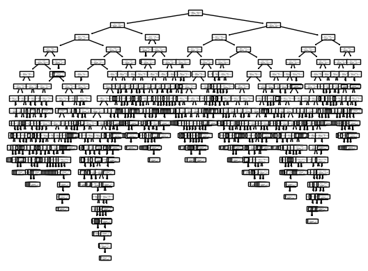
- graphviz 시각화
dot_data = tree.export_graphviz(decision_tree = model,
                                feature_names = iris.feature_names,
                                class_names = iris.target_names,
                                filled = True, rounded = True,
                                special_characters = True)
graph = graphviz.Source(dot_data)
graph
- 회귀식 시각화
plt.figure(figsize = (16, 8))

for pairidx, pair in enumerate([0, 1, 2]):
    X = diabetes.data[:, pair].reshape(-1, 1)
    y = diabetes.target

    model = DecisionTreeRegressor()
    model.fit(X, y)

    X_test = np.arange(min(X), max(X), 0.1)[:, np.newaxis]
    predict = model.predict(X_test)

    plt.subplot(1, 3, pairidx + 1)
    plt.scatter(X, y, s = 20, edgecolors = 'k', c = 'darkorange', label = 'data')
    plt.plot(X_test, predict, color = 'royalblue', linewidth = 2)
    plt.xlabel(diabetes.feature_names[pair])
    plt.ylabel('Target')
- max_depth를 3으로 줬을 때

'Python > Machine Learning' 카테고리의 다른 글
| [머신러닝 알고리즘] XGBoost, LightGBM (0) | 2023.02.23 |
|---|---|
| [머신러닝 알고리즘] 앙상블 (0) | 2023.02.18 |
| [머신러닝 알고리즘] 서포트 벡터 머신 (0) | 2023.01.13 |
| [머신러닝 알고리즘] 나이브 베이즈 (0) | 2023.01.10 |
| [머신러닝 알고리즘] K 최근접 이웃 (0) | 2023.01.10 |