● 과대적합, 과소적합을 막기 위한 방법들
- 모델의 크기 축소
- 초기화
- 옵티마이저
- 배치 정규화
- 규제화
1. 모델의 크기 축소
- 가장 단순한 방법
- 모델의 크기를 줄인다는 것은 학습 파라미터의 수를 줄이는 것
# 데이터 준비
from tensorflow.keras.datasets import imdb
import numpy as np

(train_data, train_labels), (test_data, test_labels) = imdb.load_data(num_words = 10000)

def vectorize_seq(seqs, dim = 10000):
    results = np.zeros((len(seqs), dim))
    for i, seq in enumerate(seqs):
        results[i, seq] = 1.

    return results

x_train = vectorize_seq(train_data)
x_test = vectorize_seq(test_data)

y_train = np.asarray(train_labels).astype('float32')
y_test = np.asarray(test_labels).astype('float32')
# 모델1
import tensorflow as tf
from tensorflow.keras.models import Sequential
from tensorflow.keras.layers import Dense
model_1 = Sequential([Dense(16, activation = 'relu', input_shape = (10000, ), name = 'input'),
Dense(16, activation = 'relu', name = 'hidden'),
Dense(1, activation = 'sigmoid', name = 'output')])
model_1.summary()
# 출력 결과
Model: "sequential_2"
_________________________________________________________________
Layer (type) Output Shape Param #
=================================================================
input (Dense) (None, 16) 160016
hidden (Dense) (None, 16) 272
output (Dense) (None, 1) 17
=================================================================
Total params: 160,305
Trainable params: 160,305
Non-trainable params: 0
_________________________________________________________________# 모델2
model_2 = Sequential([Dense(7, activation = 'relu', input_shape = (10000, ), name = 'input2'),
Dense(7, activation = 'relu', name = 'hidden2'),
Dense(1, activation = 'sigmoid', name = 'output2')])
model_2.summary()
# 출력 결과
odel: "sequential_3"
_________________________________________________________________
Layer (type) Output Shape Param #
=================================================================
input2 (Dense) (None, 7) 70007
hidden2 (Dense) (None, 7) 56
output2 (Dense) (None, 1) 8
=================================================================
Total params: 70,071
Trainable params: 70,071
Non-trainable params: 0
_________________________________________________________________- 모델1과 모델2 차이점은 모델의 크기 차이
# 모델 학습
model_1.compile(optimizer = 'rmsprop',
                loss = 'binary_crossentropy',
                metrics = ['acc'])
model_2.compile(optimizer = 'rmsprop',
                loss = 'binary_crossentropy',
                metrics = ['acc'])

model_1_hist = model_1.fit(x_train, y_train,
                           epochs = 20,
                           batch_size = 512,
                           validation_data = (x_test, y_test))
model_2_hist = model_2.fit(x_train, y_train,
                           epochs = 20,
                           batch_size = 512,
                           validation_data = (x_test, y_test))
# 비교
epochs = range(1, 21)
model_1_val_loss = model_1_hist.history['val_loss']
model_2_val_loss = model_2_hist.history['val_loss']
import matplotlib.pyplot as plt
plt.plot(epochs, model_1_val_loss, 'r+', label = 'Model_1')
plt.plot(epochs, model_2_val_loss, 'bo', label = 'Model_2')
plt.xlabel('Epochs')
plt.ylabel('Validation Loss')
plt.legend()
plt.grid()
plt.show()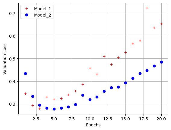
- model_2(더 작은 모델)이 조금 더 나중에 과대적합 발생
2. 모델의 크기 축소(2)
# 모델 구성
model_3 = Sequential([Dense(1024, activation = 'relu', input_shape = (10000, ), name = 'input3'),
                      Dense(1024, activation = 'relu', name = 'hidden3'),
                      Dense(1, activation = 'sigmoid', name = 'output3')])

model_3.compile(optimizer = 'rmsprop',
                loss = 'binary_crossentropy',
                metrics = ['acc'])

model_3.summary()

# 출력 결과
Model: "sequential_5"
_________________________________________________________________
 Layer (type)                Output Shape              Param #
=================================================================
 input3 (Dense)              (None, 1024)              10241024

 hidden3 (Dense)             (None, 1024)              1049600

 output3 (Dense)             (None, 1)                 1025

=================================================================
Total params: 11,291,649
Trainable params: 11,291,649
Non-trainable params: 0
_________________________________________________________________
# 모델 학습
model_3_hist = model_3.fit(x_train, y_train,
epochs = 20,
batch_size = 512,
validation_data = (x_test, y_test))# 시각화
model_3_val_loss = model_3_hist.history['val_loss']
plt.plot(epochs, model_1_val_loss, 'r+', label = 'Model_1')
plt.plot(epochs, model_2_val_loss, 'r+', label = 'Model_2')
plt.plot(epochs, model_3_val_loss, 'r+', label = 'Model_3')
plt.xlabel('Epochs')
plt.ylabel('Validation Loss')
plt.legend()
plt.grid()
plt.show()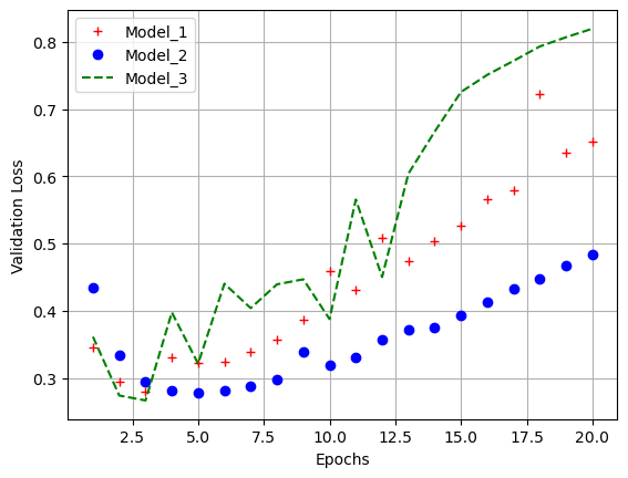
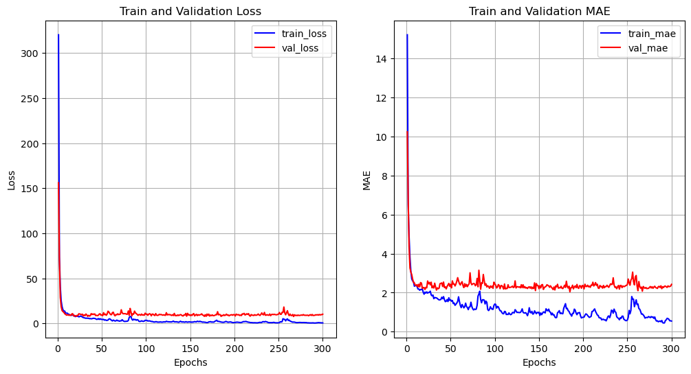
- 볼륨이 큰 신경망일수록 빠르게 훈련데이터 모델링 가능(학습 손실이 낮아짐)
- 과대적합에는 더욱 민감해짐
- 이는 학습-검증 데이터의 손실을 보면 알 수 있음
# 학습 데이터의 loss 값도 비교
model_1_train_loss = model_1_hist.history['loss']
model_2_train_loss = model_2_hist.history['loss']
model_3_train_loss = model_3_hist.history['loss']

plt.plot(epochs, model_1_train_loss, 'r+', label = 'Model_1')
plt.plot(epochs, model_2_train_loss, 'r+', label = 'Model_2')
plt.plot(epochs, model_3_train_loss, 'r+', label = 'Model_3')
plt.xlabel('Epochs')
plt.ylabel('Training Loss')
plt.legend()
plt.grid()
plt.show()
3. 가중치 초기화
- 초기화 전략
- Glorot Initialization(Xavier)
- 활성화 함수
- 없음
- tanh
- sigmoid
- softmax
- 활성화 함수
- He Initialization
- 활성화 함수
- ReLU
- LeakyReLU
- ELU 등
- 활성화 함수
from tensorflow.keras.layers import Dense, LeakyReLU, Activation
from tensorflow.keras.models import Sequential

model = Sequential([Dense(30, kernel_initializer = 'he_normal', input_shape = [10, 10]),
                    LeakyReLU(alpha = 0.2),
                    Dense(1, kernel_initializer = 'he_normal'),
                    Activation('softmax')])
model.summary()

# 출력 결과
Model: "sequential_6"
_________________________________________________________________
 Layer (type)                Output Shape              Param #
=================================================================
 dense (Dense)               (None, 10, 30)            330

 leaky_re_lu (LeakyReLU)     (None, 10, 30)            0

 dense_1 (Dense)             (None, 10, 1)             31

 activation (Activation)     (None, 10, 1)             0

=================================================================
Total params: 361
Trainable params: 361
Non-trainable params: 0
_________________________________________________________________
4. 고속 옵티마이저
- 모멘텀 최적화
$$ v \leftarrow \alpha v - \gamma \frac{\partial L}{\partial W} $$
$$ W \leftarrow W + v $$
- \(\alpha\): 관성계수
- \(v\): 속도
- \(\gamma\): 학습률
- \(\frac{\partial L}{\partial W}\): 손실함수에 대한 미분
import tensorflow as tf
from tensorflow.keras.optimizers import SGD

# momentum 값이 관성계수(알파값)
optimizer = SGD(learning_rate = 0.001, momentum = 0.9)
- 네스테로프(Nesterov)
- 모멘텀의 방향으로 조금 앞선 곳에서 손실함수의 미분을 구함
- 시간이 지날수록 조금 더 빨리 최솟값에 도달
\(m \leftarrow \beta m - \eta \bigtriangledown_{\theta}J(\theta + \beta m)\)
\(\theta \leftarrow \theta + m\) - \(h\): 기존의 기울기를 제곱하여 더한 값
- \(\eta\): 학습률
- \(\bigtriangledown_{\theta}J(\theta)\): \(\theta\)에 대한 미분(그라디언트)

optimizer = SGD(learning_rate = 0.001, momentum = 0.9, nesterov = True)
- AdaGrad
- 보통 간단한 모델에는 효과 좋을 수는 있으나, 심층 신경망 모델에서는 사용 X(사용하지 않는 것이 좋은 것으로 밝혀짐)
\(h \leftarrow h+\frac{\partial L}{\partial W} \odot \frac{\partial L}{\partial W}\)
\(W \leftarrow W+\gamma \frac{1}{\sqrt{h}} \frac{\partial L}{\partial W}\) - \(h\): 기존의 기울기를제곱하여 더한 값
- \(\gamma\): 학습률
- \(\frac{\partial L}{\partial W}\): \(W\)에 대한 미분
from tensorflow.keras.optimizers import Adagrad

optimizer = Adagrad(learning_rate = 0.001)
- RMSprop
$$ s \leftarrow \beta s+(1-\beta)\bigtriangledown_{\theta}J(\theta) \otimes \bigtriangledown_{\theta}J(\theta) $$
$$ \theta \leftarrow \theta - \eta \bigtriangledown_{\theta}J(\theta)\oslash \sqrt{s+\epsilon} $$
- \(s\): 그라디언트의 제곱을 감쇠율을 곱한 후 더함
- \(\eta\): 학습률
- \(\bigtriangledown_{\theta}J(\theta)\): 손실함수의 미분값
from tensorflow.keras.optimizers import RMSprop

optimizer = RMSprop(learning_rate = 0.001, rho = 0.9)
- Adam
$$ m \leftarrow \beta_{1}m-(1-\beta_{1})\frac{\partial L}{\partial W} $$
$$ s \leftarrow \beta_{2}s+(1-\beta_{2}\frac{\partial L}{\partial W}\odot\frac{\partial L}{\partial W} $$
$$ \hat{m} \leftarrow \frac{m}{1-\beta^{t}_{1}} $$
$$ \hat{s} \leftarrow \frac{s}{1-\beta^{t}_{2}} $$
$$ W \leftarrow W+\gamma \hat{m} \oslash \sqrt{\hat{s}+\epsilon} $$
- \(\beta\): 지수 평균의 업데이트 계수
- \(\gamma\): 학습률
- \(\beta_{1} \approx 0.9, \beta_{2} \approx 0.999 \)
- \( \frac{\partial L}{\partial W} \): \(W\)에 대한 미분
from tensorflow.keras.optimizers import Adam

# beta_1과 beta_2에 지정한 값은 디폴트 값으로, 어느정도 가장 좋은 값이라고 증명된 값
optimizer = Adam(learning_rate = 0.001, beta_1 = 0.9, beta_2 = 0.999)
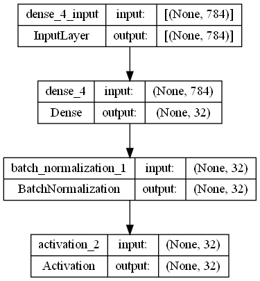
5. 배치 정규화
- 모델에 주입되는 샘플들을 균일하게 만드는 방법
- 학습 후 새로운 데이터에 잘 일반화 할 수 있도록 도와줌
- 데이터 전처리 단계에서 진행해도 되지만 정규화가 되어서 layer에 들어갔다는 보장이 없음
- 주로 Dense 또는 Conv2D Layer 후, 활성화 함수 이전에 놓임
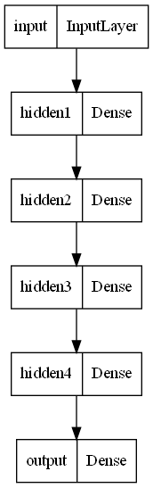
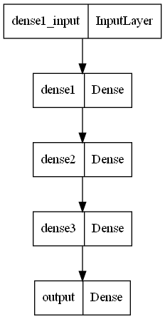
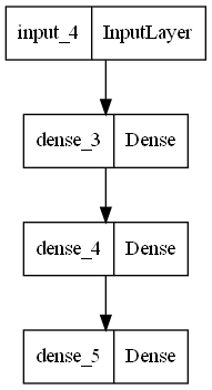
from tensorflow.keras.layers import BatchNormalization, Dense, Activation
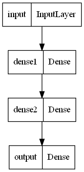
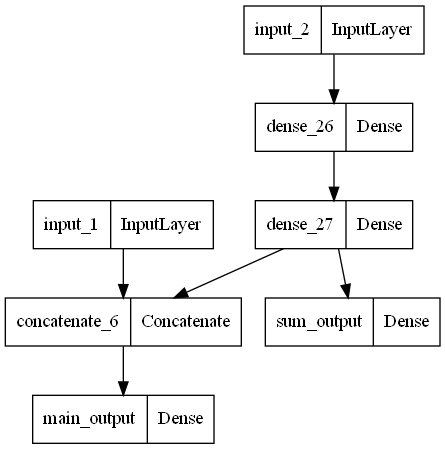
from tensorflow.keras.utils import plot_model
model = Sequential()
model.add(Dense(32, input_shape = (28 * 28, ), kernel_initializer = 'he_normal'))
model.add(BatchNormalization())
model.add(Activation('relu'))
model.summary()
plot_model(model, show_shapes = True)
# 출력 결과
Model: "sequential_9"
_________________________________________________________________
Layer (type) Output Shape Param #
=================================================================
dense_4 (Dense) (None, 32) 25120
batch_normalization_1 (Batc (None, 32) 128
hNormalization)
activation_2 (Activation) (None, 32) 0
=================================================================
Total params: 25,248
Trainable params: 25,184
Non-trainable params: 64
_________________________________________________________________
6. 규제화
- 복잡한 네트워크 일수록 네트워크 복잡도에 제한을 두어 가중치가 작은 값을 가지도록 함
- 가중치의 분포가 더 균일하게 됨
- 네트워크 손실함수에 큰 가중치에 연관된 비용을 추가
- L1 규제: 가중치의 절댓값에 비례하는 비용이 추가
- L2 규제: 가중치의 제곱에 비례한느 비용이 추가(흔히 가중치 감쇠라고도 불림)
- 위의 두 규제가 합쳐진 경우도 존재
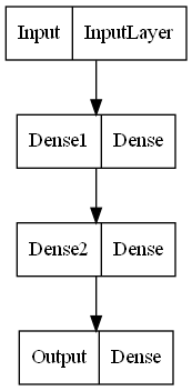
# l2 모델 구성
from tensorflow.keras.regularizers import l1, l2, l1_l2

l2_model = Sequential([Dense(16, kernel_regularizer = l2(0.001), activation = 'relu', input_shape = (10000, )),
                       Dense(16, kernel_regularizer = l2(0.001), activation = 'relu'),
                       Dense(1, activation = 'sigmoid')])
l2_model.compile(optimizer = 'rmsprop',
                 loss = 'binary_crossentropy',
                 metrics = ['acc'])
l2_model.summary()
plot_model(l2_model, show_shapes = True)

# 출력 결과
Model: "sequential_10"
_________________________________________________________________
 Layer (type)                Output Shape              Param #
=================================================================
 dense_5 (Dense)             (None, 16)                160016

 dense_6 (Dense)             (None, 16)                272

 dense_7 (Dense)             (None, 1)                 17

=================================================================
Total params: 160,305
Trainable params: 160,305
Non-trainable params: 0
_________________________________________________________________
# l2 모델 학습
l2_model_hist = l2_model.fit(x_train, y_train,
                             epochs = 20,
                             batch_size = 512,
                             validation_data = (x_test, y_test))
# l2 모델 시각화
l2_model_val_loss = l2_model_hist.history['val_loss']
epochs = range(1, 21)
plt.plot(epochs, model_1_val_loss, 'r+', label = 'Model_1')
plt.plot(epochs, l2_model_val_loss, 'bo', label = 'Model_L2-regularized')
plt.xlabel('Epochs')
plt.ylabel('Validation Loss')
plt.legend()
plt.grid()
plt.show()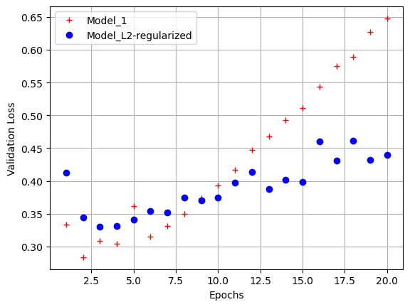
# l1 모델 구성
l1_model = Sequential([Dense(16, kernel_regularizer = l1(0.001), activation = 'relu', input_shape = (10000, )),
                       Dense(16, kernel_regularizer = l1(0.001), activation = 'relu'),
                       Dense(1, activation = 'sigmoid')])
l1_model.compile(optimizer = 'rmsprop',
                 loss = 'binary_crossentropy',
                 metrics = ['acc'])
l1_model.summary()
plot_model(l1_model, show_shapes = True)


# 출력 결과
Model: "sequential_17"
_________________________________________________________________
 Layer (type)                Output Shape              Param #
=================================================================
 dense_14 (Dense)            (None, 16)                160016

 dense_15 (Dense)            (None, 16)                272

 dense_16 (Dense)            (None, 1)                 17

=================================================================
Total params: 160,305
Trainable params: 160,305
Non-trainable params: 0
_________________________________________________________________
# l1 모델 학습
l1_model_hist = l1_model.fit(x_train, y_train,
                             epochs = 20,
                             batch_size = 512,
                             validation_data = (x_test, y_test))
# l1 모델 시각화
l1_model_val_loss = l1_model_hist.history['val_loss']
epochs = range(1, 21)
plt.plot(epochs, model_1_val_loss, 'r+', label = 'Model_1')
plt.plot(epochs, l1_model_val_loss, 'bo', label = 'Model_L1-regularized')
plt.plot(epochs, l2_model_val_loss, 'g--', label = 'Model_L2-regularized')
plt.xlabel('Epochs')
plt.ylabel('Validation Loss')
plt.legend()
plt.grid()
plt.show()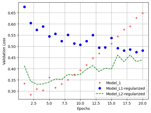
# l1_l2 모델 구성
l1_l2_model = Sequential([Dense(16, kernel_regularizer = l1_l2(l1 = 0.0001, l2 = 0.0001), activation = 'relu', input_shape = (10000, )),
                          Dense(16, kernel_regularizer = l1_l2(l1 = 0.0001, l2 = 0.0001), activation = 'relu'),
                          Dense(1, activation = 'sigmoid')])
l1_l2_model.compile(optimizer = 'rmsprop',
                    loss = 'binary_crossentropy',
                    metrics = ['acc'])
l1_l2_model.summary()
plot_model(l1_l2_model, show_shapes = True)

# 출력 결과
l1_l2_model = Sequential([Dense(16, kernel_regularizer = l1_l2(l1 = 0.0001, l2 = 0.0001), activation = 'relu', input_shape = (10000, )),
                          Dense(16, kernel_regularizer = l1_l2(l1 = 0.0001, l2 = 0.0001), activation = 'relu'),
                          Dense(1, activation = 'sigmoid')])
l1_l2_model.compile(optimizer = 'rmsprop',
                    loss = 'binary_crossentropy',
                    metrics = ['acc'])
l1_l2_model.summary()
plot_model(l1_l2_model, show_shapes = True)

# l1_l2 모델 학습
l1_l2_model_hist = l1_l2_model.fit(x_train, y_train,
                                   epochs = 20,
                                   batch_size = 512,
                                   validation_data = (x_test, y_test))
# l1_l2 모델 시각화
l1_l2_model_val_loss = l1_l2_model_hist.history['val_loss']
epochs = range(1, 21)
plt.plot(epochs, model_1_val_loss, 'r+', label = 'Model_1')
plt.plot(epochs, l1_l2_model_val_loss, 'ko', label = 'Model_L1_L2-regularized')
plt.plot(epochs, l1_model_val_loss, 'bo', label = 'Model_L1-regularized')
plt.plot(epochs, l2_model_val_loss, 'g--', label = 'Model_L2-regularized')
plt.xlabel('Epochs')
plt.ylabel('Validation Loss')
plt.legend()
plt.grid()
plt.show()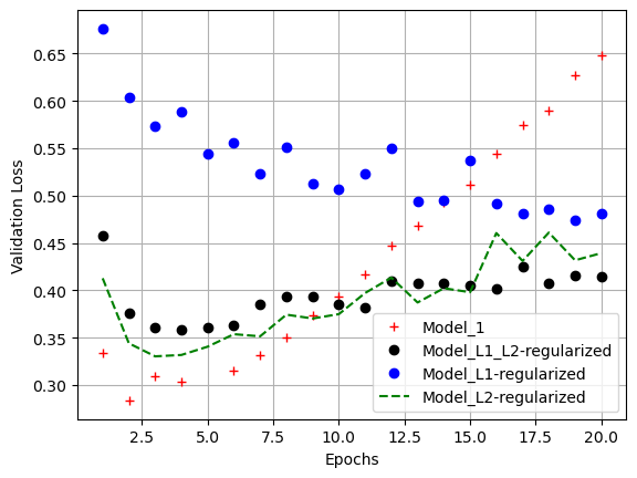
7. 드롭아웃(Dropout)
- 신경망을 위해 사용되는 규제 기법 중 가장 효과적이고 널리 사용되는 방법
- 신경망의 레이어에 드롭아웃을 적용하면 훈련하는 동안 무작위로 층의 일부 특성(노드)를 제외
- 예를 들어, 벡터 [1.0, 3.2, 0.6, 0.8, 1.1]에 대해 드롭아웃을 적용하면 무작위로 0으로 바뀜
([0, 3.2, 0.6, 0.8, 0]과 같이 바뀜) - 보통 0.2~0.5 사이의 비율로 지정됨
- 예를 들어, 벡터 [1.0, 3.2, 0.6, 0.8, 1.1]에 대해 드롭아웃을 적용하면 무작위로 0으로 바뀜
- 테스트 단계에서는 그 어떤 노드도 드롭아웃 되지 않음
- 대신 해당 레이어의 출력 노드를 드롭아웃 비율에 맞게 줄여줌
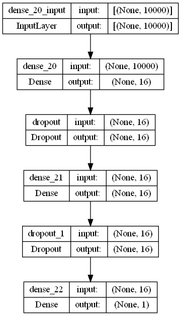
# 모델 구성
from tensorflow.keras.layers import Dropout

dropout_model = Sequential([Dense(16, activation = 'relu', input_shape = (10000, )),
                             Dropout(0.5),
                             Dense(16, activation = 'relu'),
                             Dropout(0.5),
                             Dense(1, activation = 'sigmoid')])
dropout_model.compile(optimizer = 'rmsprop',
                      loss = 'binary_crossentropy',
                      metrics = ['acc'])
dropout_model.summary()
plot_model(dropout_model, show_shapes = True)

# 출력 결과
Model: "sequential_19"
_________________________________________________________________
 Layer (type)                Output Shape              Param #
=================================================================
 dense_20 (Dense)            (None, 16)                160016

 dropout (Dropout)           (None, 16)                0

 dense_21 (Dense)            (None, 16)                272

 dropout_1 (Dropout)         (None, 16)                0

 dense_22 (Dense)            (None, 1)                 17

=================================================================
Total params: 160,305
Trainable params: 160,305
Non-trainable params: 0
_________________________________________________________________
# 모델 학습
dropout_model_hist = dropout_model.fit(x_train, y_train,
                                       epochs = 20,
                                       batch_size = 512,
                                       validation_data = (x_test, y_test))
# 시각화
dropout_model_val_loss = dropout_model_hist.history['val_loss']
epochs = range(1, 21)
plt.plot(epochs, model_1_val_loss, 'r+', label = 'Model_1')
plt.plot(epochs, dropout_model_val_loss, 'co', label = 'Model_Dropout')
plt.xlabel('Epochs')
plt.ylabel('Validation Loss')
plt.legend()
plt.grid()
plt.show()
'Python > Deep Learning' 카테고리의 다른 글
| [딥러닝-케라스] 케라스 컨볼루션 신경망 (0) | 2023.05.13 |
|---|---|
| [딥러닝-텐서플로우] 텐서플로우 Data API (1) | 2023.05.12 |
| [딥러닝-케라스] 케라스 Fashion MNIST 모델 (0) | 2023.05.08 |
| [딥러닝-케라스] 케라스 자동차 연비 예측 모델 (0) | 2023.04.28 |
| [딥러닝-케라스] 케라스 보스턴 주택 가격 모델 (0) | 2023.04.28 |