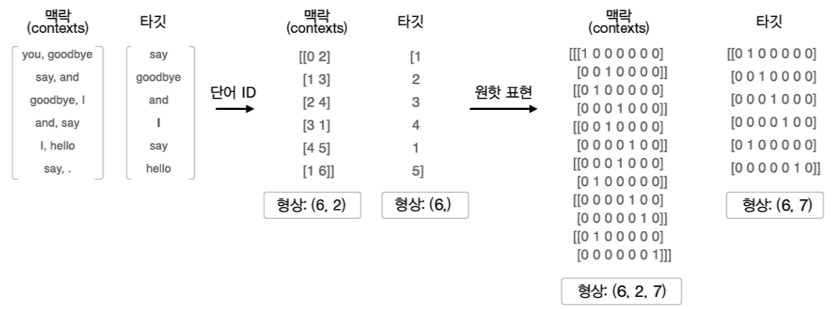
1. RNN(Recurrent Neural Network), 순환 신경망

  • 특징
    • 데이터가 순환하면서 정보가 끊임없이 갱신됨
    • 과거의 정보를 기억하는 동시에 최신 데이터로 갱신


  • 수식: \( h_{t}=tanh(h_{t-1}W_{h}+x_{t}W_{x}+b) \)
    \( W_{x} \): x를 출력 h로 변환하기 위한 가중치
    \( W_{h} \): 1개의 RNN 출력을 다음 시각의 출력으로 변환하기 위한 가중치


  - BPTT(Back Propagation Through Time)

  • 정의: RNN의 오차역전파법

  • 긴 시계열 데이터를 학습할 때 문제가 발생
    • 과도한 메모리 사용량
    • 기울기 값이 조금씩 작아지고, 0이 되어 소멸할 수 있음
    • 문제 해결을 위해 Truncated BPTT 사용


  - Truncated BPTT

  • 기능: 신경망을 적당한 지점에서 잘라내어 작은 신경망 여러 개로 만듦

  • 역전파의 연결은 끊어지지만, 순전파의 연결은 끊어지지 않음

위쪽의 순전파에서는 h9에서 h9로 이어지지만 역전파에서는 중간에 끊어짐


  - 미니배치 학습

  • 미니배치를 나눠서 사용할 때 순서 고려
  • 예시) 길이가 1000인 데이터에 대해 시각의 길이를 10개 단위로 잘라서 Truncated BPTT로 학습하는 경우
    • 첫번째 미니배치의 원소는 0~9, 두번째 미니배치의 원소는 500~509
    • 다음 순서는 10~19, 510~519로, 학습 처리 순서를 고려해서 미니배치의 순서 고려


  - Time RNN

  • RNN의 연속된 형태를 Time RNN이라는 하나의 형태로 만들어냄


  - RNN 순전파

class RNN:
    def __init__(self, Wx, Wh, b):
        self.params = [Wx, Wh, b]
        self.grads = [np.zeros_like(Wx), np.zeros_like(Wh), np.zeros_like(b)]
        self.cache = None
    
    def forward(self, x, h_prev):
        Wx, Wh, b = self.params
        t = np.dot(h_prev, Wh) + np.dot(x, Wx) + b
        h_next = np.tanh(t)

        self.cache = (x, h_prev, h_next)
        return h_next


  - RNN 역전파

  - Time RNN 구현

  • 은닉 상태의 h를 인스턴스 변수를 인계받는 용도로 이용

  • Time RNN 순전파
class TimeRNN:
    def __init__(self, Wx, Wh, b, stateful = False):
        self.params = [Wx, Wh, b]
        self.grads = [np.zeros_like(Wx), np.zeros_like(Wh), np.zeros_like(b)]
        self.layers = None

        # h: 마지막 RNN 계층의 h 저장
        # dh: 앞 블록의 기울기 저장
        self.h, self.dh = None, None
        self.stateful = stateful

    def forward(self, xs):
        Wx, Wh, b = self.params
        # N: 미니배치 크기
        # T: T개 분량의 시계열 데이터
        # D: 차원수
        N, T, D = xs.shape
        D, H = Wx.shape

        self.layers = []

        # hs: 출력값을 담을 그릇(N, T, H만큼의 빈공간을 만들어 둠)
        hs = np.empty((N, T, H), stype = 'f')

        # 처음 시작 시 초기화
        if not self.stateful or self.h is None:
            self.h = np.zeros((N, H), dtype = 'f')
        
        for t in range(T):
            layer = RNN(*self.params)
            self.h = layer.forward(xs[:, t, :], self.h)
            hs[:, t, :] = self.h
            self.layers.append(layer)

        return hs
  • Time RNN 역전파

class TimeRNN:
    ...
    
    def backward(self, dhs):
        Wx, Wh, b = self.params
        N, T, H = dhs.shape
        D, H = Wx.shape

        # 입력데이터 기울기 정보 저장
        dxs = np.empty((N, T, D), dtype = 'f')
        dh = 0
        grads = [0, 0, 0]
        for t in reversed(range(T)):
            layer = self.layers[t]

            # layer.backward(): 입력 데이터 기울기, 이전 h 기울기 반환
            dx, dh = layer.backward(dhs[:, t, :] + dh)
            dxs[:, t, :] = dx

            for i, grad in enumerate(layer.grads):
                grads[i] += grad
        
        for i, grad in enumerate(grads):
            self.grads[i][...] = grad
        self.dh = dh

        return dxs


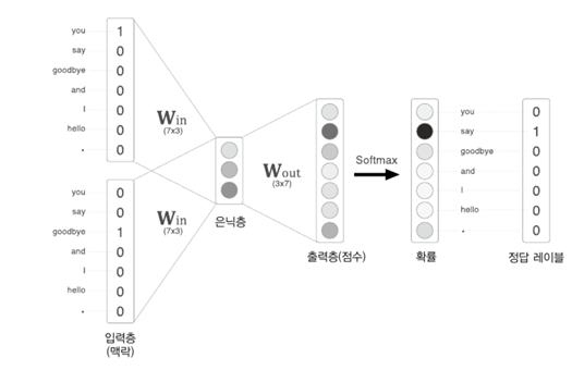
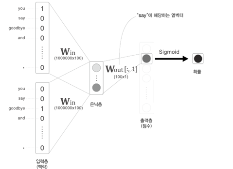
  - RNNLM(RNN Language Model)

  • RNN을 사용한 언어 모델

왼쪽: RNNLM의 계층 구성 / 오른쪽: 계층 구성을 시간축으로 펼친 신경망

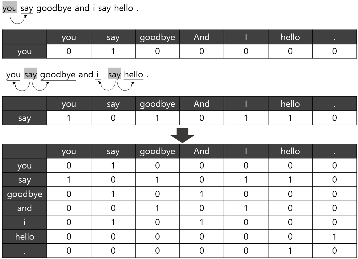
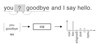
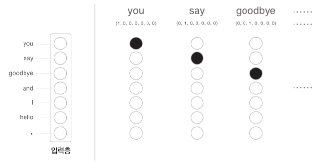
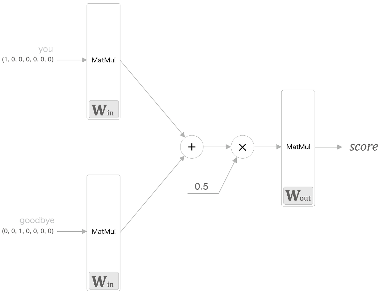
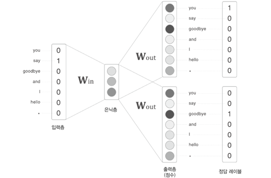
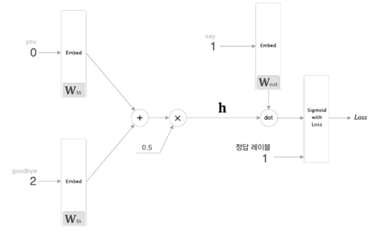
  • 샘플 말뭉치('You say goodbye and I say hello.')를 처리하는 

입력 데이터: 단어 ID의 배열

  1. 첫번째 시각
    • 첫 단어로 단어 ID가 0인 'you' 입력
    • 이때 softmax 계층이 출력하는 확률분포는 'say'가 가장 높음
      • 즉, 'you' 다음에 출현하는 단어가 'say'라는 것을 올바르게 예측
      • 이처럼 제대로 예측하려면 좋은 가중치(잘 학습된 가중치)를 사용해야 함
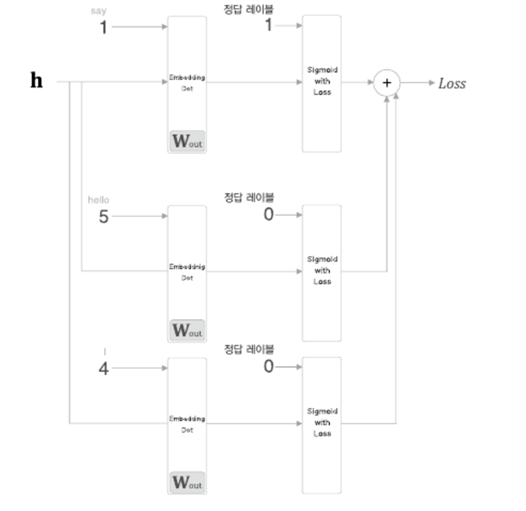
  2. 두번째 시각
    • 두번째 단어로 'say'가 입력
    • softmax 계층 출력은 'goodbye'와 'hello'가 높음
      • 'you say goodbye'와 'you say hello'는 모두 자연스러움
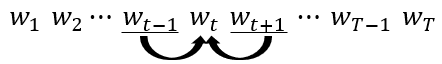
  3. 주목할 점
    • RNN 계층은 'you say'라는 맥락을 기억하고 있음
    • RNN은 'you say'라는 과거의 정보를 응집된 은닉 상태 벡터로 저장해두고 있음
      • 그러한 정보를 더 위의 Affine 계층에, 그리고 다음 시각의 RNN 계층에 전달하는 것이 RNN 계층이 하는 일


  - Time Affine 계층

  • 시간에 따른 변화를 한번에 나타내는 것으로 만들 수 있음
    • 각 시각의 Embedding을 합쳐서 Time Embedding으로
    • 각 시각의 RNN을 합쳐서 Time RNN으로
    • 각 시각의 Affine을 합쳐서 Time Affine으로
    • 각 시각의 Softmax을 합쳐서 Time Softmax로


  - 시계열 버전의 softmax

  • softmax 계층을 구현할 때는 손실 오차를 구하는 Cross Entropy Error 계층도 함께 구현
  • 여기서 Time Softmax with Loss 계층으로 구현

softmax loss 구현 수식: 전체 Loss 값을 다 더한 후 T로 나누어 평균 구하기


  - RNNLM 구현

from common.time_layers import TimeEmbedding, TimeAffine
class SimpleRnnlm:
    def __init__(self, vocab_size, wordvec_size, hidden_size):
        V, D, H = vocab_size, wordvec_size, hidden_size
        rn = np.random.randn

        # 가중치 초기화
        embed_W = (rn(V, D) / 100).astype('f')
        rnn_Wx = (rn(D, H) / np.sqrt(D)).astype('f')
        rnn_Wh = (rn(H, H) / np. sqrt(H)).astype('f')
        rnn_b = np.zeros(H).astype('f')
        affine_W = (rn(H, V) / np.sqrt(H)).astype('f')
        affine_b = np.zeros(V).astype('f')

        # 계층 생성
        self.layers = [
            TimeEmbedding(embed_W),
            TimeRNN(rnn_Wx, rnn_Wh, rnn_b, stateful = True),
            TimeAffine(affine_W, affine_b)
        ]


  - 퍼플렉서티(Perplexity)

  • 기능: 언어 모델의 예측 성능 평가
  • 수식: 확률의 역수
  • 특징: 작을수록 예측을 잘한 것으로 판별

RNNLM 결과를 Perplexity를 활용하여 나타낸 그래프


2. 게이트가 추가된 RNN

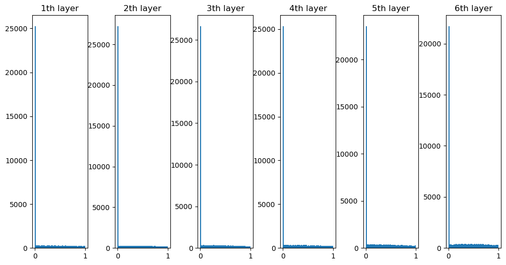
  • RNN의 문제점: 길이가 길어지면 기울기가 소실되면 장기 의존 관계를 학습할 수 없음

  • 기울기 소실과 기울기 폭발의 원인
    • y=tanh(x) 그래프에서 x가 0으로부터 멀어질수록 값이 작아짐

    • 매번 똑같은 가중치 \( W_{h} \)를 사용

기울기 폭발
기울기 소실


  • 기울기 폭발 대책: clipping
    \( if \left || \hat{g} \right || \geq threshold \)
    \( \hat{g} = \frac{threshold}{\left || \hat{g} \right ||} \hat{g} \)
import numpy as np

dW1 = np.random.rand(3, 3) * 10
dW2 = np.random.rand(3, 3) * 10
grads = [dW1, dW2]
max_norm = 5.0

def clip_grads(grads, max_norm):
    total_norm = 0
    for grad in grads:
        total_norm += np.sum(grad ** 2)
    total_norm = np.sqrt(total_norm)

    rate = max_norm / (total_norm + 1e-6)
    if rate < 1:
        for grad in grads:
            grad *= rate

print('before:', dW1.flatten())
clip_grads(grads, max_norm)
print('after:', dW1.flatten())

# 출력 결과
before: [0.292 1.409 1.208 5.685 0.065 9.458 2.011 0.732 7.078]
after: [0.069 0.335 0.288 1.353 0.015 2.251 0.479 0.174 1.685]


  • 기울기 소실과 LSTM
    • RNN을 LSTM으로 바꾸면 새로운 c라는 경로가 생김
    • c는 메모리셀을 의미, LSTM의 기억을 위한 셀

  • LSTM(Long Short Term Memory): 길게 기억할건지, 짧게 기억할건지 흐름을 조절


  • LSTM의 output 게이트
    • c값을 고려

[1]
입력 \( x_{t} \) 에는 가중치 \( (W_{x})^{(0)} \)가,
이전 시각의 은닉 상태 \( h_{t}-1 \) 에는 가중치 \( (W_{h})^{(0)} \)가 붙어있음 (\( x_{t} \)  \( h_{t}-1 \)은 행벡터)

[2]
그리고 이 행렬들의 곱과 편향 \( b^{(o)} \)를 모두 더한 다음

[3]
시그모이드 함수를 거쳐 출력 게이트의 출력 o를 구함.

[4]
마지막으로 이 o와 \( tanh(c_{t}) \)의 원소별 곱을 \( h_{t} \) 로 출력

output 게이트에서 수행하는 계산을‘σ’로 표기
그리고 σ의 출력을 o라고 하면, \( h_{t} \) 는 \( o \)와 \(tanh(c_{t}) \)의 곱으로 계산된다.

  • 여기서 말하는 ‘곱’이란 원소별 곱
  • 이것을 아다마르 곱 Hadamard product 이라고 함.


  • tanh의 출력은 -1.0~1.0의 실수
  • 이 -1.0~1.0의 수치를 그 안에 인코딩된 ‘정보’의 강약(정도)을 표시한다고 해석할 수 있음
  • 한편 시그모이드 함수의 출력은 0.0~1.0의 실수이며, 데이터를 얼마만큼 통과시킬지를 정하는 비율
    • (주로) 게이트에서는 시그모이드 함수가
    • 실질적인 ‘정보’를 지니는 데이터에는 tanh 함수가 활성화 함수로 사용됨


  • LSTM의 forget 게이트: 불필요한 기억을 잊게 해주는 부분
  • LSTM의 새로운 기억 셀(g)


  • LSTM 기울기 흐름: 메모리인 c에 어떤 정보가 전달되는지가 중요(잊을 건 잊고, 유지될 건 유지되어 전달되는 형태)


  - LSTM 구현

  • 수식 구현

  • 구현한 수식을 하나로 모으면 아래와 같이 표현 가능(Affine 변환)

from common.functions import sigmoid

class LSTM:
    def __init__(self, Wx, Wh, b):

        self.params = [Wx, Wh, b]
        self.grads = [np.zeros_like(Wx), np.zeros_like(Wh), np.zeros_like(b)]
        self.cache = None
    
    def forward(self, x, h_prev, c_prev):
        Wx, Wh, b = self.params
        N, H = h_prev.shape

        A = np.dot(x, Wx) + np.dot(h_prev, Wh) + b

        f = A[:, :H]
        g = A[:, H:2*H]
        i = A[:, 2*H:3*H]
        o = A[:, 3*H:]

        f = sigmoid(f)
        g = np.tanh(g)
        i = sigmoid(i)
        o = sigmoid(o)

        c_next = f * c_prev + g * i
        h_next = o * np.tanh(c_next)

        self.cache = (x, h_prev, c_prev, i, f, g, o, c_next)
        return h_next, c_next
    
    def backward(self, dh_next, dc_next):
        Wx, Wh, b = self.params
        x, h_prev, c_prev, i, f, g, o, c_next = self.cache

        tanh_c_next = np.tanh(c_next)

        ds = dc_next + (dh_next * o) * (1 - tanh_c_next ** 2)

        dc_prev = ds * f

        di = ds * g
        df = ds * c_prev
        do = dh_next * tanh_c_next
        dg = ds * i

        di *= i * (1 - i)
        df *= f * (1 - f)
        do *= o * (1 - o)
        dg *= (1 - g ** 2)

        dA = np.hstack((df, dg, di, do))

        dWh = np.dot(h_prev.T, dA)
        dWx = np.dot(x.T, dA)
        db = dA.sum(axis=0)

        self.grads[0][...] = dWx
        self.grads[1][...] = dWh
        self.grads[2][...] = db

        dx = np.dot(dA, Wx.T)
        dh_prev = np.dot(dA, Wh.T)

        return dx, dh_prev, dc_prev

  1. 처음 4개분의 아핀 변환을 한꺼번에 수행
  2. 그리고 slice 노드를 통해 그 4개의 결과를 꺼냄
    • slice: 아핀 변환의 결과(행렬)를 균등하게 네조각으로 나눠서 꺼내주는 단순한 노드
  3. slice 노드 다음에는 활성화 함수(시그모이드 함수 또는 tanh 함수)를 거쳐 앞 절에서 설명한 계산을 수행


  • slice 노드의 역전파: 이 slice 노드는 행렬을 네 조각으로 나눠서 분배
    → 따라서 그 역전파에서는 반대로 4 개의 기울기 결합 필요


  - Time LSTM 구현

from common.functions import sigmoid

class TimeLSTM:
    def __init__(self, Wx, Wh, b, stateful = False):

        self.params = [Wx, Wh, b]
        self.grads = [np.zeros_like(Wx), np.zeros_like(Wh), np.zeros_like(b)]
        self.cache = None

        self.h , self.c = None, None
        self.dh = None
        self.statful = stateful
    
    def forward(self, xs):
        Wx, Wh, b = self.params
        N, T, D = xs.shape
        H = Wh.shape[0]

        self.layers = []
        hs = np.empty((N, T, H), dtype = 'f')

        if not self.stateful or self.h is None:
            self.h = np.zeros((N, H), dtype = 'f')
        if not self.stateful or self.c is None:
            self.c = np.zeros((N, H), dtype = 'f')
        
        for t in range(T):
            layer = LSTM(*self.params)
            self.h, self.c = layer.forward(xs[:, t, :], self.h, self.c)
            hs[:, t, :] = self.h
            
            self.layers.appen(layer)
        
        return hs
    
    def backward(self, dhs):
        Wx, Wh, b = self.params
        N, T, H = dhs.shape
        D = Wx.shape[0]

        dxs = np.empty((N, T, D), dtype = 'f')
        dh, dc = 0, 0

        grads = [0, 0, 0]
        for t in reversed(range(T)):
            layer = self.layers[t]
            dx, dh, dc = layer.backward(dhs[:, t, :] + dh, dc)
            dxs[:, t, :] = dx
            for i, grad in enumerate(layer.grads):
                grads[i] = grad
        
        for i, grad in enumerate(grads):
            self.grads[i][...] = grad
        self.dh = dh
        return dxs
    
    def set_state(self, h, c = None):
        self.h, self.c = h, C

    def reset_state(self):
        self.h, self.c = None, None


  - RNNLM 구현

from common.time_layers import TimeSoftmaxWithLoss

class Rnnlm:
    def __init__(self, vocab_size = 10000, wordvec_size = 100, hidden_size = 100):

        V, D, H = vocab_size, wordvec_size, hidden_size
        rn = np.random.randn

        # 가중치 초기화
        embed_W = (rn(V, D) / 100).astype('f')
        lstm_Wx = (rn(D, 4 * H) / np.sqrt(D)).astype('f')
        lstm_Wh = (rn(H, 4 * H) / np.sqrt(H)).astype('f')
        lstm_b = np.zeros(4 * H).astype('f')
        affine_W = (rn(H, V) / np.sqrt(H)).astype('f')
        affine_b = np.zeros(V).astype('f')

        # 계층 생성
        self.layers = [
            TimeEmbedding(embed_W),
            TimeRNN(lstm_Wx, lstm_Wh, lstm_b, stateful=True),
            TimeAffine(affine_W, affine_b)
        ]
        self.loss_layer = TimeSoftmaxWithLoss()
        self.rnn_layer = self.layers[1]

        # 모든 가중치와 기울기를 리스트에 모음
        self.params, self.grads = [], []
        for layer in self.layers:
            self.params += layer.params
            self.grads += layer.grads
    
    def predict(self, xs):
        for layer in self.layers:
            xs = layer.forward(xs)
        return xs

    def forward(self, xs, ts):
        score = self.predict(xs)
        loss =self.loss_layer.forward(score, ts)
        return loss

    def backward(self, dout=1):
        dout = self.loss_layer.backward(dout)
        for layer in reversed(self.layers):
            dout = layer.backward(dout)
        return dout

    def reset_state(self):
        self.rnn_layer.reset_state()
  • 모델 동작 결과 - 장기적으로 기억하고 잊어버릴 건 잊어버리는 게이트 역할을 LSTM이 해줌으로써 더 좋은 성능 출력
from common.optimizer import SGD
from common.trainer import RnnlmTrainer
from common.util import eval_perplexity

# 하이퍼파라미터 설정
batch_size = 20
wordvec_size = 100
hidden_size = 100  # RNN의 은닉 상태 벡터의 원소 수
time_size = 35     # RNN을 펼치는 크기
lr = 20.0
max_epoch = 4
max_grad = 0.25

# 학습 데이터 읽기
corpus, word_to_id, id_to_word = ptb.load_data('train')
corpus_test, _, _ = ptb.load_data('test')
vocab_size = len(word_to_id)
xs = corpus[:-1]
ts = corpus[1:]

# 모델 생성
model = Rnnlm(vocab_size, wordvec_size, hidden_size)
optimizer = SGD(lr)
trainer = RnnlmTrainer(model, optimizer)

# 기울기 클리핑을 적용하여 학습
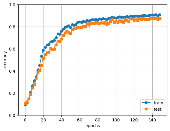
trainer.fit(xs, ts, max_epoch, batch_size, time_size, max_grad,
            eval_interval=20)
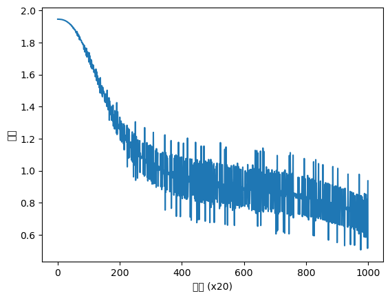
trainer.plot(ylim=(0, 500))

# 테스트 데이터로 평가
model.reset_state()
ppl_test = eval_perplexity(model, corpus_test)
print('테스트 퍼플렉서티: ', ppl_test)

# 매개변수 저장
model.save_params()

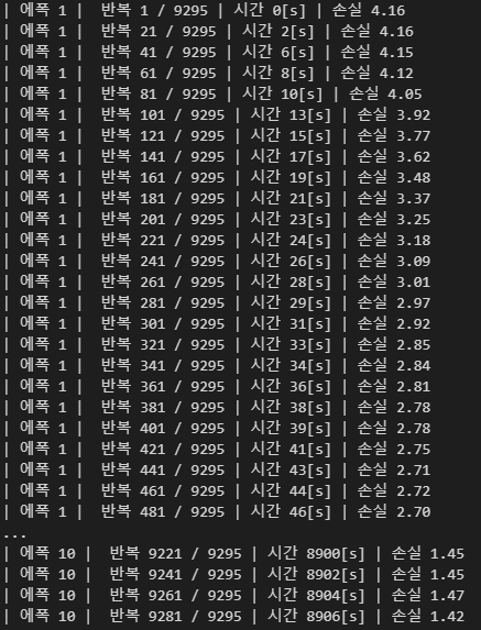
퍼플렉서티 평가 중 ... 234 / 235 테스트 퍼플렉서티: 135.88121947675342


  - RNNLM의 추가 개선: LSTM 계층 다양화

  • LSTM 계층을 깊게 쌓아(계층을 여러겹 쌓아) 효과를 볼 수 있음

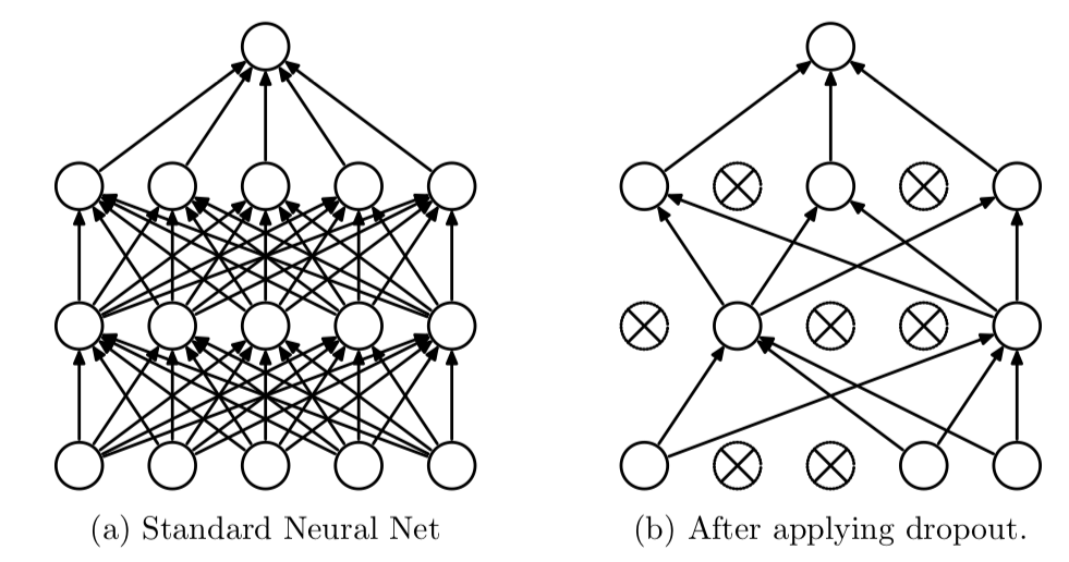
  - RNNLM의 추가 개선: 드롭아웃에 의한 과적합 억제

  • 망의 일부만 계산에 사용

  • 드롭아웃 계층의 삽입 위치(나쁜 예): LSTM 계층의 시계열 방향으로 삽입
    • 시계열 방향으로 드롭아웃 학습 시, 흐름에 따라 정보가 사라질 수 있음(흐르는 시간에 비례해 드롭아웃에 의한 노이즈 축적)

  • 드롭아웃 계층의 삽입 위치(좋은 예): 드롭아웃 계층을 깊이 방향(상하 방향)으로 삽입
    • 시간 방향(좌우 방향)으로 아무리 진행해도 정보를 잃지 않음
    • 드롭아웃이 시간축과는 독립적으로 깊이 방향에만 영향을 줌

  • 변형 드롭아웃: 깊이 방향은 물론 시간 방향에도 사용가능, 언어 모델의 정확도 향상


  - RNNLM의 추가 개선: 가중치 공유

  • Embedding의 가중치와 Affine의 가중치를 공유하며
    • 매개변수 수가 줄어들고
    • 정확도 향상


  - 개선된 RNNLM 구현

from common.time_layers import *
import numpy as np
from common.base_model import BaseModel

class BetterRnnlm(BaseModel):
    def __init__(self, vocab_size=10000, wordvec_size=650,
                 hidden_size=650, dropout_ratio=0.5):
        V, D, H = vocab_size, wordvec_size, hidden_size
        rn = np.random.randn

        # LSTM 계층 2개 사용
        # 각 층에 드롭아웃 적용
        embed_W = (rn(V, D) / 100).astype('f')
        lstm_Wx1 = (rn(D, 4 * H) / np.sqrt(D)).astype('f')
        lstm_Wh1 = (rn(H, 4 * H) / np.sqrt(H)).astype('f')
        lstm_b1 = np.zeros(4 * H).astype('f')
        lstm_Wx2 = (rn(H, 4 * H) / np.sqrt(H)).astype('f')
        lstm_Wh2 = (rn(H, 4 * H) / np.sqrt(H)).astype('f')
        lstm_b2 = np.zeros(4 * H).astype('f')
        affine_b = np.zeros(V).astype('f')

        self.layers = [
            TimeEmbedding(embed_W),
            TimeDropout(dropout_ratio),
            TimeLSTM(lstm_Wx1, lstm_Wh1, lstm_b1, stateful=True),
            TimeDropout(dropout_ratio),
            TimeLSTM(lstm_Wx2, lstm_Wh2, lstm_b2, stateful=True),
            TimeDropout(dropout_ratio),
            # 가중치 공유
            TimeAffine(embed_W.T, affine_b)
        ]
        self.loss_layer = TimeSoftmaxWithLoss()
        self.lstm_layers = [self.layers[2], self.layers[4]]
        self.drop_layers = [self.layers[1], self.layers[3], self.layers[5]]

        self.params, self.grads = [], []
        for layer in self.layers:
            self.params += layer.params
            self.grads += layer.grads

    def predict(self, xs, train_flg=False):
        for layer in self.drop_layers:
            layer.train_flg = train_flg

        for layer in self.layers:
            xs = layer.forward(xs)
        return xs

    def forward(self, xs, ts, train_flg=True):
        score = self.predict(xs, train_flg)
        loss = self.loss_layer.forward(score, ts)
        return loss

    def backward(self, dout=1):
        dout = self.loss_layer.backward(dout)
        for layer in reversed(self.layers):
            dout = layer.backward(dout)
        return dout

    def reset_state(self):
        for layer in self.lstm_layers:
            layer.reset_state()
  • 구현된 모델 학습
# 하이퍼파라미터 설정
batch_size = 20
wordvec_size = 650
hidden_size = 650
time_size = 35
lr = 20.0
max_epoch = 40
max_grad = 0.25
dropout = 0.5

# 학습 데이터 읽기
corpus, word_to_id, id_to_word = ptb.load_data('train')
corpus_val, _, _ = ptb.load_data('val')
corpus_test, _, _ = ptb.load_data('test')

if config.GPU:
    corpus = to_gpu(corpus)
    corpus_val = to_gpu(corpus_val)
    corpus_test = to_gpu(corpus_test)

vocab_size = len(word_to_id)
xs = corpus[:-1]
ts = corpus[1:]

model = BetterRnnlm(vocab_size, wordvec_size, hidden_size, dropout)
optimizer = SGD(lr)
trainer = RnnlmTrainer(model, optimizer)

best_ppl = float('inf')
for epoch in range(max_epoch):
    trainer.fit(xs, ts, max_epoch=1, batch_size=batch_size,
                time_size=time_size, max_grad=max_grad)

    model.reset_state()
    ppl = eval_perplexity(model, corpus_val)
    print('검증 퍼플렉서티: ', ppl)

    if best_ppl > ppl:
        best_ppl = ppl
        model.save_params()
    else:
        lr /= 4.0
        optimizer.lr = lr

    model.reset_state()
    print('-' * 50)


# 테스트 데이터로 평가
model.reset_state()
ppl_test = eval_perplexity(model, corpus_test)
print('테스트 퍼플렉서티: ', ppl_test)

  • 시간은 오래 걸리지만
    개선된 모델에서는 퍼플렉서티 감소

1. 자연어 처리

  • 자연어(Natural Language): 한국어와 영어 등 우리가 평소에 쓰는 말
  • 자연어 처리(Natural Language Processing, NLP): 언어를 컴퓨터에게 이해시키기 위한 기술
  • 단어의 의미를 잘 파악하는 표현 방법
    • 시소러스를 활용한 기법
    • 통계 기반 기법
    • 추론 기반 기법(word2vec)


  - 시소러스(Thesaurus)

  • 시소러스: 유의어 사전
    • 동의어나 유의어가 한 그룹으로 분류
    • 상·하위, 전체와 부분 등의 관계까지 정의
  • 모든 단어가 레이블링 되어 있다면, '단어 네트워크'를 이용하여 컴퓨터에게 단어 사이의 관계를 가르칠 수 있음
    • ex) WordNet, K-Thesaurus 등
  • 시소러스의 문제점
    • 시대 변화에 대응하기 어려움
    • 사람이 쓰는 비용이 큼
    • 단어의 미묘한 차리를 표현할 수 없음


  - 통계 기반 기법

  • 어떤 단어에 주목했을 때, 그 주변에 어떤 단어가 몇 번이나 등장하는지를 세어 집계하는 방법
  • ex) 검색 기반 방법혼이 발전 되어 나온 방법
    - 번역 데이터를 모으는 일은 쉬운 일이 아니며 보통은 1천만 문장쌍이 있어야 쓸만한 성능이 나옴
    - 도메인(분야: 뉴스, 특허, 웹채팅, SNS 등)에 굉장히 의존적이며 뉴스 도메인 데이터로 학습한 모델을 SMS 번역에 적용하면 심각한 성능저하 발생
import numpy as np

def preprocess(text):
    text = text.lower()
    text = text.replace('.', ' .')
    words = text.split(' ')

    word_to_id = {}
    id_to_word = {}
    for word in words:
        if word not in word_to_id:
            new_id = len(word_to_id)
            word_to_id[word] = new_id
            id_to_word[new_id] = word
    
    corpus = np.array([word_to_id[w] for w in words])
    return corpus, word_to_id, id_to_word

text = 'You say goodbye and I say hello.'
corpus, word_to_id, id_to_word = preprocess(text)
print('corpus:' + str(corpus))
print('word_to_id:' + str(word_to_id))
print('id_to_word:' + str(id_to_word))

# 출력 결과
# say는 첫 say에서 id가 1번으로 부여되어 뒤에 나온 say에 새로운 id 부여없이 1로 사용
corpus:[0 1 2 3 4 1 5 6]
word_to_id:{'you': 0, 'say': 1, 'goodbye': 2, 'and': 3, 'i': 4, 'hello': 5, '.': 6}
id_to_word:{0: 'you', 1: 'say', 2: 'goodbye', 3: 'and', 4: 'i', 5: 'hello', 6: '.'}
  • 파이썬으로 말뭉치 전처리하기
  • 단어의 분산 표현
    • '단어의 의미'를 정확하게 파악할 수 있는 벡터 표현
    • 단어를 고정 길이의 '밀집벡터'로 표현
    • 밀집벡터: 대부분의 원소가 0이 아닌 실수인 벡터 (ex/ (R, G, B) = (170, 33, 22))
  • 분포 가설
    • 단어의 의미는 주변 단어에 의해 형성
    • 단어 자체에는 의미가 없고, 그 단어가 사용된 '맥락'이 의미를 형성
    • 맥락: 주목하는 단어 주변에 놓인 단어
    • 맥락의 크기(주변 단어를 몇 개나 포함할 지) = 윈도우 크기
  • 동시발생 행렬

def create_co_matrix(corpus, vocab_size, window_size = 1):
    corpus_size = len(corpus)
    co_matrix = np.zeros((vocab_size, vocab_size), dtype = np.int32)

    for idx, word_id in enumerate(corpus):
        for i in range(1, window_size + 1):
            left_idx = idx - i
            right_idx = idx + i
            
            if left_idx >= 0:
                left_word_id = corpus[left_idx]
                co_matrix[word_id, left_word_id] += 1
            
            if right_idx < corpus_size:
                right_word_id = corpus[right_idx]
                co_matrix[word_id, right_word_id] += 1
    
    return co_matrix
C = create_co_matrix(corpus, len(word_to_id))
C

# 출력 결과
array([[0, 1, 0, 0, 0, 0, 0, 0],
           [1, 0, 1, 0, 1, 1, 0, 0],
           [0, 1, 0, 1, 0, 0, 0, 0],
           [0, 0, 1, 0, 1, 0, 0, 0],
           [0, 1, 0, 1, 0, 0, 0, 0],
           [0, 1, 0, 0, 0, 0, 1, 0],
           [0, 0, 0, 0, 0, 1, 0, 0],
           [0, 0, 0, 0, 0, 0, 0, 0]])


  • 벡터 간 유사도
    • 벡터의 내적, 유클리드 거리등
    • 코사인 유사도(cosine similarity)를 자주 이용

$$ similarity(x, y) = \frac{x \cdot y}{\left || x \right || \left || y \right ||} = \frac{x_{1}y_{1} + \cdots + x_{n}y_{n}}{\sqrt{x_{1}^{2} + \cdots + x_{n}^{2}} \sqrt{y_{1}^{2} + \cdots + y_{n}^{2}}} $$

def cos_similarity(x, y, eps = 1e-8):
    nx = x / np.sqrt(np.sum(x**2) + eps)
    ny = y / np.sqrt(np.sum(y**2) + eps)
    return np.dot(nx, ny)

c0 = C[word_to_id['you']]  # 'you'의 단어 벡터: [0 1 0 0 0 0 0]
c1 = C[word_to_id['i']]  # 'i'의 단어 벡터: [0 1 0 1 0 0 0]
print(cos_similarity(c0, c1))

# 출력 결과
0.7071067758832467


  - 통계 기반 기법 개선하기

  • 유사 단어 랭킹 표시
def most_similar(query, word_to_id, id_to_word, word_matrix, top = 5):
    if query not in word_to_id:
        print("'%s(을)를 찾을 수 없습니다."%query)
        return
    print('\n[query]'+query)

    query_id = word_to_id[query]
    query_vec = word_matrix[query_id]

    vocab_size = len(id_to_word)
    similarity = np.zeros(vocab_size)
    for i in range(vocab_size):
        similarity[i] = cos_similarity(word_matrix[i], query_vec)

    count = 0
    for i in (-1*similarity).argsort():
        if id_to_word[i] == query:
            continue
        print('%s: %s'%(id_to_word[i], similarity[i]))

        count += 1
        if count >= top:
            return
most_similar('he', word_to_id, id_to_word, C, top = 5)

# 출력 결과
'he(을)를 찾을 수 없습니다.
most_similar('you', word_to_id, id_to_word, C, top = 5)

# 출력 결과
[query]you
goodbye: 0.7071067758832467
i: 0.7071067758832467
hello: 0.7071067758832467
say: 0.0
and: 0.0
  • 직관적으로 'you' & 'hello', 'you' & 'goodbye'는 관련이 없어 보일 수 있음
  • 이는 말뭉치의 크기가 너무 작기 때문


  • 상호정보량(점별 상호정보량(Pointwise Mutual Information, PMI)
    \( PMI(x, y) = log_{2} \frac{P(x, y)}{P(x)P(y)} = log_{2} \frac{\frac{C(x, y)}{N}}{\frac{C(x)}{N}\frac{C(y)}{N}}=log_{2}\frac{C(x, y) \cdot N}{C(x)C(y)} \)
    • x, y가 일어날 확률 / x가 일어날 확률, y가 일어날 확률
    • 양의 상호정보량(Positive PMI, PPMI)
      \( PPMI(x, y)=max(0, PMI(x, y)) \)
def ppmi(C, verbose = False, eps = 1e-8):
    M = np.zeros_like(C, dtype = np.float32)
    N = np.sum(C)
    S = np.sum(C, axis = 0)
    total = C.shape[0] * C.shape[1]
    cnt = 0

    for i in range(C.shape[0]):
        for j in range(C.shape[1]):
            pmi = np.log2(C[i, j] * N / (S[i] * S[j]) + eps)
            M[i, j] = max(0, pmi)

            if verbose:
                cnt += 1
                if cnt % (total //100) == 0:
                    print('%.1f%% 완료'%(100 * cnt / total))
    return M

C = create_co_matrix(corpus, len(word_to_id), window_size = 1)
W = ppmi(C)

np.set_printoptions(precision = 3)
print("동시발생 행렬")
print(C)
print('-'*50)
print('PPMI')
print(W)

# 출력 결과
동시발생 행렬
[[0 1 0 0 0 0 0]
 [1 0 1 0 1 1 0]
 [0 1 0 1 0 0 0]
 [0 0 1 0 1 0 0]
 [0 1 0 1 0 0 0]
 [0 1 0 0 0 0 1]
 [0 0 0 0 0 1 0]]
--------------------------------------------------
PPMI
[[0.    1.807 0.    0.    0.    0.    0.   ]
 [1.807 0.    0.807 0.    0.807 0.807 0.   ]
 [0.    0.807 0.    1.807 0.    0.    0.   ]
 [0.    0.    1.807 0.    1.807 0.    0.   ]
 [0.    0.807 0.    1.807 0.    0.    0.   ]
 [0.    0.807 0.    0.    0.    0.    2.807]
 [0.    0.    0.    0.    0.    2.807 0.   ]]
  • PPMI 행렬의 문제점
    • 말뭉치의 어휘수가 증가함에 따라 단어 벡터의 차원 수도 증가
    • 원소 대부분이 0(각 원소의 중요도가 낮음
    • 노이즈에 약하고 견고하지 못함
    → 중요한 정보는 최대한 유지하면서 차원을 줄여야 함


  • 차원 감소 - 특이값 분해(Singular Value Decomopsition, SVD)

full SVD
thin SVD
compact SVD
truncated SVD

import sys
sys.path.append('..')
import numpy as np
import matplotlib.pyplot as plt

text = "You say goodbye and I say hello."
corpus, word_to_id, id_to_word = preprocess(text)
vocab_size= len(word_to_id)
C = create_co_matrix(corpus, vocab_size)
W = ppmi(C)
U, S, V = np.linalg.svd(W)

print('차원 감소된 U')
print(U[:, :2])

for word, word_id in word_to_id.items():
    plt.annotate(word, (U[word_id, 0], U[word_id, 1]))
plt.scatter(U[:, 0], U[:, 1], alpha = 0.5)
plt.show()

# 출력 결과
차원 감소된 U
[[-1.110e-16  3.409e-01]
 [-5.976e-01  0.000e+00]
 [-5.551e-17  4.363e-01]
 [-4.978e-01  1.665e-16]
 [-3.124e-17  4.363e-01]
 [-3.124e-17  7.092e-01]
 [-6.285e-01 -1.943e-16]]


2. Word2Vec

  • 단어를 벡터로 표현하는 방법
    • 통계 기반 기법: 배치학습(많은 데이터를 한번에 처리), 학습 데이터에 대해 SVD을 통해 저차원으로 변환
    • 추론 기반 기법: 미니 배치 학습 가능(전체를 다 하지 않고 필요한 부분만 분리시켜 학습, 나눠서 처리하므로 나눠서 할 수 있고 GPU 병렬 계산 등이 가능)


  - 신경망에서의 단어 처리

  • 추론 기반 기법의 주된 작업은 추론
  • 모델로 사용하는 것은 신경망
  • '?'를 추론하기 위해 맥락을 모델에 넣어 '?' 자리에 올 수 있는 단어의 확률분포 값을 추론해서 알려줌 


  • 신경망은 단어를 그대로 처리할 수 없음
  • 원-핫 표현으로 변환(벡터의 원소 중 하나만 1이고 나머지는 모두 0인 벡터
  • 신경망의 입력층은 뉴런의 수 고정


  • 단어 하나를 완전연결계층을 통해 변환
    • 완전연결계층: 인접하는 계층의 모든 뉴런과 연결되어 있는 신경망


  • C와 W의 곱은 가중치의 행벡터 한 줄과 같음
  • matmul로도 수행가능
import numpy as np

c = np.array([1, 0, 0, 0, 0, 0, 0]) # 입력
W = np.random.randn(7, 3)  # 가중치
h = np.matmul(c,W)  # 중간 노드
print(h)

# 출력 결과
[-0.473 -1.132 -1.333]


  - CBOW(continuous bag-of-word) 모델

  • 주변 단어들로부터 중앙 단어를 추측하는 용도의 신경망
  • CBOW의 입력은 맥락
  • 맥락에 포함시킬 단어가 N개면 입력층도 N개
  • 입력층이 여러 개일 경우 은닉층은 전체의 평균을 하면 됨
  • 출력층에 소프트맥스 함수를 적용하여 확률을 얻을 수 있음

  • 계층  관점에서 CBOW 모델의 신경망 구성
    • you와 goodbye 사이에 무엇이 올지 추론
    • 가중치 계산할 때 행렬곱한 뒤, 0.5를 곱함(두 개의 평균을 취하기 위해)
    • 그 후 가중치 출력을 통해 점수를 계산

import numpy as np
from common.layers import MatMul

c0 = np.array([[1, 0, 0, 0, 0, 0 ,0]])
c1 = np.array([[0, 0, 1, 0, 0, 0, 0]])

W_in = np.random.randn(7, 3)
W_out = np.random.randn(3, 7)

in_layer0 = MatMul(W_in)
in_layer1 = MatMul(W_in)
out_layer = MatMul(W_out)

h0 = in_layer0.forward(c0)
h1 = in_layer1.forward(c1)
h = 0.5 * (h0 + h1)
s = out_layer.forward(h)
print(s)

# 출력 결과
[[ 0.216  0.096  0.06   0.536  0.389 -0.392 -0.217]]
  • CBOW 모델의 학습에서 하는 일: 올바른 학습을 할 수 있게 가중치 조절
  • 다루고 있는 모델은 다중 클래스 분류를 수행하는 신경망(softmax와 cross entropy error)만 이용하면 됨


  - word2vec의 가중치와 분산 표현

  • Word2vec에서 사용되는 가중치는 2개가 존재
    • W(in) 입력층 완전 연결계층의 가중치
    • W(out) 출력층 완전 연결계층의 가중치
  • 최종적으로 이용하는 단어의 분산표현으로는 어느 가중치를 선택해야 할까?
    → 가장 대중적인 선택: W(in) 입력층 완전 연결계층의 가중치만 이용하는 것


  - 맥락과 타겟

  • 타겟: 맥락에 둘러 싸인 중앙의 단어(정답 레이블)
  • 말뭉치 → 단어 ID 변환

def create_contexts_target(corpus, window_size = 1):
    # 문장의 첫단어부터 마지막 단어까지가 타겟
    target = corpus[window_size:- window_size]
    contexts = []

    for idx in range(window_size, len(corpus) - window_size):
        cs = []
        for t in range(-window_size, window_size + 1):
            if t == 0:
                continue
            cs.append(corpus[idx + t])
        contexts.append(cs)
    return np.array(contexts), np.array(target)

contexts, target = create_contexts_target(corpus, window_size = 1)
print(contexts)
print(target)
# 출력 결과
[[0 2]
 [1 3]
 [2 4]
 [3 1]
 [4 5]
 [1 6]]
[1 2 3 4 1 5]


  • 맥락과 타겟 → 원-핫 표현으로 변환

def convert_one_hot(corpus, vocab_size):
    N = corpus.shape[0]

    if corpus.ndim == 1:
        one_hot = np.zeros((N, vocab_size), dtype = np.int32)
        for idx, word_id in enumerate(corpus):
            one_hot[idx, word_id] = i
    
    elif corpus.ndim == 2:
        C = corpus.shape[1]
        one_hot = np.zeros((N, C, vocab_size), dtype = np.int32)
        for idx_0, word_ids in enumerate(corpus):
            for idx_1, word_id in enumerate(word_ids):
                one_hot[idx_0, idx_1, word_id] = 1
    
    return one_hot


  - CBOW 모델 구현

  • 생성자레서 어휘 수와 뉴런 수를 입력 받음
  • 가중치 두 개 생성
    • astype(f): float형으로 타입 변환
  • MatMul 계층 2개, 출력층 1개, Softmax with Loss 계층 1개 생성
  • 매개변수와 기울기를 인스턴스 변수에 모음
  • 이때 사용한 common.layers import SoftmaxWithLoss 파일은 '밑바닥부터 시작하는 딥러닝' github에서 다운받음
    https://github.com/WegraLee/deep-learning-from-scratch-2 )
from common.layers import MatMul
from common.layers import SoftmaxWithLoss

class SimpleCBOW:
    def __init__(self, vocab_size, hidden_size):
        V, H = vocab_size, hidden_size

        # 가중치 초기화
        W_in = 0.01 * np.random.randn(V, H).astype('f')
        W_out = 0.01 * np.random.randn(H, V).astype('f')

        # 계층 생성
        self.in_layer0 = MatMul(W_in)
        self.in_layer1 = MatMul(W_in)
        self.out_layer = MatMul(W_out)
        self.loss_layer = SoftmaxWithLoss()

        # 모든 가중치와 기울기를 리스트에 모으기
        layers = [self.in_layer0, self.in_layer1, self.out_layer]
        self.params, self.grads = [], []
        for layer in layers:
            self.params += layer.params
            self.grads += layer.grads

        # 인스턴스 변수에 단어의 분산 표현 저장
        self.word_vecs = W_in
    
    def forward(self, contexts, target):
        h0 = self.in_layer0.forward(contexts[:, 0])
        h1 = self.in_layer1.forward(contexts[:, 1])
        h = (h0 + h1) * 0.5
        score = self.out_layer.forward(h)
        loss = self.loss_layer.forward(score, target)

        return loss
    
    def backward(self, dout = 1):
        ds = self.loss_layer.backward(dout)
        da = self.out_layer.backward(ds)
        da *= 0.5
        self.in_layer1.backward(da)
        self.in_layer0.backward(da)
        return None

  • 학습코드 구현
from common.trainer import Trainer
from common.optimizer import Adam

window_size = 1
hidden_size = 5
batch_size = 3
max_epoch = 1000

text = 'You say goodbye and I say hello.'
corpus, word_to_id, id_to_word = preprocess(text)

vocab_size = len(word_to_id)
contexts, target = create_contexts_target(corpus, window_size)
target = convert_one_hot(target, vocab_size)
contexts = convert_one_hot(contexts, vocab_size)

model = SimpleCBOW(vocab_size, hidden_size)
optimizer = Adam()
trainer = Trainer(model, optimizer)

trainer.fit(contexts, target, max_epoch, batch_size)
trainer.plot()

word_vecs = model.word_vecs
for word_id, word in id_to_word.items():
    print(word, word_vecs[word_id])


  - word2vec 보충

  • 동시확률: A와 B가 동시에 일어날 확률
  • 사후확률: 사건이 일어난 후의 확률

  • 타깃이 \( W_{t} \)가 될 확률은 수식으로
    \( P(w_{t}|w_{t-1}, w_{t+1}) \)
  • 손실함수도 간결하게 표현 가능
    \( L=-logP(w_{t}|w_{t-1}, w_{t+1}) \)
  • 말 뭉치 전체로 확장
    \( L=-\frac{1}{T}\sum_{t=1}^{T}logP(w_{t}|w_{t-1}, w_{t+1}) \)


  - skip-gram 모델

  • Word2vec은 CBOW 모델, skip-gram 모델 두 개 제안
  • skip-gram모델은 CBOW에서 다루는 맥락과 타겟을 역전시킨 모델

  • 입력층은 하나, 출력의 수는 맥락의 수만큼 존재
  • 개별 손실들을 모두 더한 값이 최종 손실이 됨

  • skip-gram 모델의 확률 표기
    • \( W_{t} \)가 주어졌을 때, \( W_{t-1} \)과 \( W_{t+1} \)이 동시에 일어날 확률
      \( P(w_{t-1}, w_{t+1}|w_{t}) \)
    • 조건부 독립
      \( P(w_{t-1}, w_{t+1}|w_{t})=P(w_{t-1}|w_{t})P(w_{t+1}|w_{t}) \)
    • skip-gram 모델의 손실 함수
      \( L=-logP(w_{t-1}, w_{t+1}|w_{t} \\ \quad =-logP(w_{t-1}|w_{t})P(w_{t+1}|w_{t}) \\ \quad =-(logP(w_{t-1}|w_{t})+logP(w_{t+1}|w_{t})) \)
    • 말뭉치 전체의 손실함수
      \( L=-\frac{1}{T} \sum_{t=1}^{T}(logP(w_{t-1}|w_{t})+logP(w_{t+1}|w_{t})) \)
  • CBOW모델과 SKip-gram모델을 비교했을 때,
    단어 분산 표현의 정밀도 면에서 skip-gram모델이 유리
    • 말뭉치가 커질수록 성능이 뛰어남
    • 학습속도는 CBOW모델보다 느림


3. Word2Vec 속도 개선

  • word2vec의 문제점: 말뭉치에 포함된 어휘 수가 많아지면 계산량도 커짐
  • word2vec의 개선방향
    • Embedding이라는 새로운 개층 도입
    • 네거티브 샘플링이라는 새로운 손실함수 도입


  - word2vec 개선 1

  • 입력측 가중치(W_in)와의 행렬곱으로 은닉층 계산
  • 출력측 가중치(W_out)와의 행렬곱으로 각 단어의 점수 구함
  • softmax 함수를 적용해 단어의 확률을 얻어 손실 구함

  • CBOW 모델의 문제점
    • 입력층의 원-핫 표현과 가중치 행렬(W_in)의 곱 계산
      → Embedding 계층을 도입해서 해결
    • 은닉층과 가중치 행렬(W_out)의 곱 및 softmax 계층의 계산
      → 네거티브 샘플링을 도입해서 해결


  - Embedding 계층

  • 맥락 c와 가중치 W의 곱으로 해당 위치의 행 벡터 추출 → 결과적으로 행렬의 특정 행을 추출하는 것

import numpy as np
W = np.arange(21).reshape(7, 3)
W

# 출력 결과
array([[ 0,  1,  2],
          [ 3,  4,  5],
          [ 6,  7,  8],
          [ 9, 10, 11],
          [12, 13, 14],
          [15, 16, 17],
          [18, 19, 20]])
W[0]

# 출력 결과
array([0, 1, 2])


W[2]

# 출력 결과
array([6, 7, 8])


idx = np.array([1, 0, 3, 0])
W[idx]

# 출력 결과
array([[ 3,  4,  5],
          [ 0,  1,  2],
          [ 9, 10, 11],
          [ 0,  1,  2]])


  • Embedding의 순전파, 역전파 구현

  • Embedding 계층 backward의 문제점
    • 아래 그림에서 첫번째와 세번째가 중복으로 0번 인덱스에 들어가야 하는데 어떻게 처리해야 하나
      → 중복문제 해결을 위해, 할당이 아닌 '더하기'를 해주어야 함

class Embedding:
    def __init__(self, W):
        self.params = [W]
        self.grads = [np.zeros_like(W)]
        self.idx = None

    def forward(self, idx):
        W = self.params
        self.idx = idx
        out = W[idx]
        return out
    
    def backward(self, dout):
        dW = self.grads
        dW[...] = 0
        
        # backward의 중복 문제 해결을 위해 더하기를 해줌
        np.add.at(dW, self.idx, dout)
        # 혹은 다음과 같은 for문 사용
        # for i, word_id in enumerate(self.idx):
        # dW[word_id] += dout[i]
        
        return None


  - word2vec 개선 2

  • 은닉층 이후에 계산이 오래 걸리는 곳(은닉측의 뉴런과 가중치 행렬(W_out)의 곱 / softmax 계층의 계산)
    (\( y_{k}=\frac{exp(s_{k}}{\sum_{i=1}^{1000000}exp(s_{i})} \))


  • 다중 분류에서 이진 분류로(네거티브 샘플링)

  • 출력층의 가중치 W_out에서는 각 단어 ID의 단어 벡터가 열로 저장되어 있음
  • 아래의 예에서 'say'에 해당하는 단어 벡터를 추출
    → 그 벡터와 은닉층 뉴런과의 내적을 구함

  다중 분류 이진 분류
출력층 softmax sigmoid
손실 함수 cross entropy error cross entropy error


  • 시그모이드 함수와 교차 엔트로피 오차
    • 시그모이드 함수
      \( y=\frac{1}{1+exp(-x)} \)
    • 교차 엔트로피 오차
      \( L=-(tlogy+(1-t)log(1-y)) \)
      t가 1이면 정답은 'Yes' → -log y 출력
      t가 1이면 정답은 'No' → -log (1-y) 출력

  • 정답 레이블이 1이라면 y가 1(100%)에 가까워질수록 오차가 줄어듦
    반대로, y가 1로부터 멀어지면 오차가 커짐
  • 오차가 크면 '크게' 학습하고, 오차가 작으면 '작게' 학습하게 됨


  • 다중 분류 구현

다중분류

  • 이진 분류 구현
    • 은닉층 뉴런 h와 출력층의 가중치 W_out에서 'say'에 해당하는 단어 벡터와의 내적을 계산
    • 출력을 Sigmoid with Loss 계층에 입력해 최종 손실을 얻음

이진분류

  • Embedding Dot 계층을 도입

class EmbeddingDot:
    def __init__(self, W):
        self.embed = Embedding(W)
        self.params = self.embed.params # 매개변수 저장
        self.grads = self.embed.grads  # 기울기 저장
        self.cache = None
    
    def forward(self, h, idx):
        target_W = self.embed.forward(idx)
        out = np.sum(target_W * h, axis = 1)  # 내적 계산

        self.cache = (h, target_W)
        return out
    
    def backward(self, dout):
        h, target_W = self.cache
        dout = dout.reshape(dout.shape[0], 1)
        
        dtarget_W = dout * h
        self.embed.backward(dtarget_W)
        dh = dout * target_W
        return dh
idx = [0, 3, 1]
embed = Embedding(W)
target_W = embed.forward(idx)
out = np.sum(target_W * h, axis = 1)

target_W

# 출력 결과
array([[ 0,  1,  2],
          [ 9, 10, 11],
          [ 3,  4,  5]])


out

# 출력 결과
array([0.383, 7.621, 2.796])

  • 정답은 1에 가깝게, 오답은 0에 가깝게 만들어야 함
  • 부정적인 예에서는 오답이 무엇인지 알 수 없음
  • 네거티브 샘플링을 통해 부정적인 예를 전부 학습하지 않고 일부만 샘플링하여 학습
    • 긍정적인 예(say): Sigmoid with Loss 계층에 정답 레이블로 '1'을 입력함
    • 부정적인 예(hello와 I): Sigmoid with Loss 계층에 정답 레이블로 '0'을 입력함


  • 네거티브 샘플링의 샘플링 기법
    • 말뭉치에서 각 단어의 출현 횟수를 구해 '확률분포'로 샘플링

import numpy as np

# 무작위 샘플링
words = ['you', 'say', 'goodbye', 'I', 'hello', '']
np.random.choice(words)

# 5개 무작위 샘플링(죽복 o)
np.random.choice(words, size = 5)

# 5개 무작위 샘플링(죽복 x)
np.random.choice(words, size = 5, replace = False)

# 확률분포에 따라 샘플링
# 아래는 각 단어가 선택될 확률
p = [0.5, 0.1, 0.05, 0.2, 0.05, 0.1]
np.random.choice(words, p = p)
  • \( P'(w_{i}-\frac{P(w_{i})^0.75}{\sum_{j}^{n}P(w_{j})^0.75} \)
  • 기본 확률분포에 0.75를 제곱하는 방법을 추천
    0.75를 제곱함으로써, 원래 확률이 낮은 단어의 확률을 살짝 높일 수 있음
p = [0.7, 0.29, 0.01]
new_p = np.power(p, 0.75)
new_p /= np.sum(new_p)
print(new_p)

# 출력 결과
[0.642 0.332 0.027]


  • UnigramSampler: 네거티브 샘플링 말뭉치에서 단어의 확률분포를 만들고, 0.75 제곱한 후 np.random.choice()를 사용해 부정적 예를 샘플링하는 클래스
# UnigramSampler 클래스
import collections
GPU=False
class UnigramSampler:
    def __init__(self, corpus, power, sample_size):
        self.sample_size = sample_size
        self.vocab_size = None
        self.word_p = None

        counts = collections.Counter()
        for word_id in corpus:
            counts[word_id] += 1

        vocab_size = len(counts)
        self.vocab_size = vocab_size

        self.word_p = np.zeros(vocab_size)
        for i in range(vocab_size):
            self.word_p[i] = counts[i]

        self.word_p = np.power(self.word_p, power)
        self.word_p /= np.sum(self.word_p)  # 전체 합이 1이 되도록 확률 설정

    def get_negative_sample(self, target):
        batch_size = target.shape[0]

        if not GPU:
            negative_sample = np.zeros((batch_size, self.sample_size), dtype=np.int32)

            for i in range(batch_size):
                p = self.word_p.copy()
                target_idx = target[i]
                p[target_idx] = 0
                p /= p.sum() # 정답 부분의 확률을 0으로 만들어 버렸으므로 남은 확률들의 합이 1이되도록 하기 위함
                negative_sample[i, :] = np.random.choice(self.vocab_size, size=self.sample_size, replace=False, p=p)
        else:
            # GPU(cupy)로 계산할 때는 속도를 우선
            # 부정적인 예에 타겟이 포함될 수 있음
            negative_sample = np.random.choice(self.vocab_size, size=(batch_size, self.sample_size),
                                               replace=True, p=self.word_p)

        return negative_sample
corpus = np.array([0, 1, 2, 3, 4, 1, 2, 3])
power = 0.75
sample_size = 2

sampler = UnigramSampler(corpus, power, sample_size)
target = np.array([1, 3, 0])
negative_sample = sampler.get_negative_sample(target)
print(negative_sample)

# 출력 결과
[[2 3]
 [0 2]
 [1 3]]


  • 네거티브 샘플링 손실함수 클래스 구현
from common.layers import SigmoidWithLoss
class NegativeSamplingLoss:
    def __init__(self, W, corpus, power = 0.75, sample_size = 5):
        self.sample_size = sample_size
        self.sampler = UnigramSampler(corpus, power, sample_size)
        self.loss_layers = [SigmoidWithLoss for _ in range(sample_size + 1)]
        self.embed_dot_layers = [EmbeddingDot(W) for _ in range(sample_size + 1)]

        self.params, self.grads = [], []
        for layer in self.embed_dot_layers:
            self.params += layer.params
            self.grads += layer.grads

    def forward(self, h, target):
        batch_size = target.shape[0]
        negative_sample = self.sampler.get_negative_sample(target)

        # 긍정적인 예 순전파
        score = self.embed_dot_layers[0].forward(h, target)
        correct_label = np.ones(batch_size, dtype = np.int32)
        loss = self.loss_layers[0].forward(score, correct_label)

        # 부정적인 예 순전파
        negative_label = np.zeros(batch_size, dtype = np.int32)
        for i in range(self.sample_size):
            negative_target = negative_sample[:, i]
            score = self.embed_dot_layers[1 + i].forward(h, negative_target)
            loss += self.loss_layers[1 + i].forward(score, negative_label)

        return loss
    
    def backward(self, dout = 1):
        dh = 0
        for I0, I1 in zip(self.loss_layers, self.embed_dot_layers):
            dscore = I0.backward(dout)
            dh += I1.backward(dscore)

        return dh


  • 개선된 word2vec 학습
import numpy as np

class CBOW:
    def __init__(self, vocab_size, hidden_size, window_size, corpus):
        V, H = vocab_size, hidden_size

        # 가중치 초기화
        W_in = 0.01 * np.random.randn(V, H).astype('f')
        W_out = 0.01 * np.random.randn(V, H).astype('f')

        # 계층 생성
        self.in_layers = []
        for i in range(2 * window_size):
            layer = Embedding(W_in)
            self.in_layers.append(layer)
        self.ns_loss = NegativeSamplingLoss(W_out, corpus, power = 0.75, sample_size = 5)

        # 모든 가중치와 기울기를 배열에 모음
        layers = self.in_layers + [self.ns_loss]
        self.params, self.grads = [], []
        for layer in layers:
            self.params += layer.params
            self.grads += layer.grads

        # 인스턴스 변수에 단어의 분산 표현 저장
        self.word_vecs = W_in

    def forward(self, contexts, target):
        h = 0
        for i, layer in enumerate(self.in_layers):
            h += layer.forward(contexts[:, i])
        h *= 1 / len(self.in_layers)
        loss = self.ns_loss.forward(h, target)
        return loss
    
    def backward(self, dout = 1):
        dout = self.ns_loss.backward(dout)
        dout *= 1 / len(self.in_layers)
        for layer in self.in_layers:
            layer.backward(dout)
        return None
# CBOW 모델 학습
from common import config
import pickle
from common.trainer import Trainer
from common.optimizer import Adam
from common.util import to_cpu, to_gpu
from dataset import ptb


window_size = 5
hidden_size = 100
batch_size = 100
max_epoch = 10

corpus, word_to_id, id_to_word = ptb.load_data('train')
vocab_size = len(word_to_id)

contexts, target = create_contexts_target(corpus, window_size)
if config.GPU:
    contexts, target = to_gpu(contexts), to_gpu(target)

model = CBOW(vocab_size, hidden_size, window_size, corpus)
optimizer = Adam()
trainer = Trainer(model, optimizer)

trainer.fit(contexts, target, max_epoch, batch_size)
trainer.plot()

word_vecs = model.word_vecs
if config.GPU:
    word_vecs = to_cpu(word_vecs)
params = {}
params['word_vecs'] = word_vecs.astype(np.float16)
params['word_to_id'] = word_to_id
params['id_to_word'] = id_to_word
pkl_file = 'cbow_params.pkl'
with open(pkl_file, 'wb') as f:
    pickle.dump(params, f, -1)


  • word2vec의 단어 분산 표현을 사용하면 유추문제를 덧셈과 뺄셈으로 풀 수 있음
    • king → ?에서 ?를 man → woman의 관계로부터 유추
    • analogy 함수 사용

# 유추 문제
from common.util import analogy

pkl_file = 'cbow_params.pkl'

with open(pkl_file, 'rb') as f:
    params = pickle.load(f)
    word_vecs = params['word_vecs']
    word_to_id = params['word_to_id']
    id_to_word = params['id_to_word']

# 가장 비슷한 단어 뽑기
querys = ['you', 'year', 'car', 'toyota']
for query in querys:
    most_similar(query, word_to_id, id_to_word, word_vecs, top = 5)

# 유추(analogy) 작업
print('-' * 50)
analogy('king', 'man', 'queen', word_to_id, id_to_word, word_vecs)
analogy('take', 'took', 'go', word_to_id, id_to_word, word_vecs)
analogy('car', 'cars', 'child', word_to_id, id_to_word, word_vecs)
analogy('good', 'better', 'bad', word_to_id, id_to_word, word_vecs)


  - 자연어 처리 분야에서 단어의 분산 표현이 중요한 이유

  • 전이 학습 가능
  • 단어를 고정 길이 벡터로 변환해줌(bag of words)


  - word2vec을 사용한 애플리케이션의 예

  • 메일 자동 분류 시스템 만들기
    1. 데이터(메일) 수집
    2. 수동으로 레이블링 작업(3단계의 감정을 나타내는 레이블)
    3. 학습된 word2vec을 이용해 메일을 벡터로 변환
    4. 감정분석을 수행하는 어떤 분류 시스템(SVM이나 신경망 등)에 벡터화된 메일과 감정 레이블을 입력하여 학습 수행


  - 단어 벡터 평가 방법

  • 모델에 따라 정확도가 다름(말뭉치에 따라 적합한 모델 선택
  • 일반적으로 말뭉치가 클수록 결과가 좋음(항상 데이터가 많은 게 좋음)
  • 단어 벡터 차원 수는 적당한 크기가 좋음(너무 커도 정확도가 나빠짐)


  - 정리

  • Embedding 계층은 단어의 분산 표현을 담고 있으며, 순전파 시 지정한 단어 ID의 벡터를 추출
  • Word2vec은 어휘 수 증가에 비례항 계산량도 증가하므로, 근사치로 계산하는 빠른 기법을 사용하면 좋음
  • 네거티브 샘플링은 부정적 예를 몇 개 샘플링한느 기법으로, 이를 이요하면 다중 분류를 이진 분류처럼 취급
  • word2vec으로 얻은 단어의 분산 표현에는 단어의 의미가 녹아들어 있으며, 비슷한 맥락에서 사용되는 단어는 벡터 공간에서 가까이 위치함
  • word2vec은 전이 학습 측면에서 특히 중요하며, 그 단어의 분산 표현은 다양한 자연어 처리 작업에 이용할 수 있음

● 합성곱 신경망 구현

1. 합성곱 층(Convolution Layer)

# 이미지를 column으로 바꿔주는 함수
def im2col(input_data, filter_h, filter_w, stride = 1, pad = 0):
    N, C, H, W = input_data.shape
    out_h = (H + 2* pad - filter_h) // stride + 1
    out_w = (W + 2* pad - filter_w) // stride + 1

    img = np.pad(input_data, [(0, 0), (0, 0), (pad, pad), (pad, pad)], 'constant')
    col = np.zeros((N, C, filter_h, filter_w, out_h, out_w))

    for y in range(filter_h):
        y_max = y + stride * out_h
        for x in range(filter_w):
            x_max = x + stride * out_w
            col[:, :, y, x, :, :] = img[:, :, y:y_max:stride, x:x_max:stride]
    
    # reshape 해줌으로써 flatten된 결과가 나옴
    col = col.transpose(0, 4, 5, 1, 2, 3).reshape(N * out_h * out_w, -1)
    return col

# column을 이미지로 바꿔주는 함수
def col2im(col, input_shape, filter_h, filter_w, stride = 1, pad = 0):
    N, C, H, W = input_shape
    out_h = (H + 2* pad - filter_h) // stride + 1
    out_w = (W + 2* pad - filter_w) // stride + 1
    col = col.reshape(N, out_h, out_w, C, filter_h, filter_w).transpose(0, 3, 4, 5, 1, 2)

    img = np.zeros((N, C, H + 2 * pad + stride - 1, W + 2 * pad + stride - 1))
    for y in range(filter_h):
        y_max = y + stride * out_h
        for x in range(filter_w):
            x_max = x + stride * out_w
            img[:, :, y:y_max:stride, x:x_max:stride] += col[:, :, y, x, :, :]
    
    return img[:, :, pad:H + pad, pad:W + pad]
# 2차원 합성곱 연산 클래스
class Conv2D:
    def __init__(self, W, b, stride = 1, pad = 0):
        self.W = W
        self.b = b
        self.stride = stride
        self.pad = pad

        self.input_data = None
        self.col = None
        self.col_W = None
        self.dW = None
        self.db = None
    
    def forward(self, input_data):
        FN, C, FH, FW = self.W.shape
        N, C, H, W = input_data.shape
        out_h = (H + 2 * self.pad - FH) // self.stride + 1
        out_w = (W + 2 * self.pad - FW) // self.stride + 1

        col = im2col(input_data, FH, FW, self.stride, self.pad)
        col_W = self.W.reshape(FN, -1).T

        out = np.dot(col, col_W) + self.b
        output = out.reshape(N, out_h, out_w, -1).transpose(0, 3, 1, 2)

        self.input_data = input_data
        self.col = col
        self.col_W = col_W

        return output
    
    def backward(self, dout):
        FN, C, FH, FW = self.W.shape
        dout = dout.reshape(0, 2, 3, 1).reshape(-1, FN)

        self.db = np.sum(dout, axis = 0)
        self.dW = np.dot(self.col.T, dout)
        self.dW = self.dW.transpose(1, 0).reshape(FN, C, FH, FW)

        dcol = np.dot(dout, self.col_W.T)
        dx = col2im(dcol, self.input_data.shape, FH, FW, self.stride, self.pad)

        return dx


  - 컨볼루션 레이어 테스트

def init_weight(num_filters, data_dim, kernel_size, stride = 1, pad = 0, weight_std = 0.01):
    weights = weight_std * np.random.randn(num_filters, data_dim, kernel_size, kernel_size)
    biases = np.zeros(num_filters)
    return weights, biases
# 기본 이미지 출력
img_url = "https://upload.wikimedia.org/wikipedia/ko/thumb/2/24/Lenna.png/440px-Lenna.png"
image_gray = url_to_image(img_url, gray = True)
image_gray = image_gray.reshape(image_gray.shape[0], -1, 1)
print("image.shape:", image_gray.shape)

image_gray = np.expand_dims(image_gray.transpose(2, 0, 1), axis = 0)

plt.imshow(image_gray[0, 0, :, :], cmap = 'gray')
plt.show()

# 가중치와 편향주어 합성곱 연산 (1)
W, b = init_weight(1, 1, 3)
conv = Conv2D(W, b)
output = conv.forward(image_gray)

print("Conv Layer size:", output.shape)

# 출력 결과
Conv Layer size: (1, 1, 438, 438)


plt.imshow(output[0, 0, :, :], cmap = 'gray')
plt.show()

# 가중치와 편향주어 합성곱 연산 (2)
W2, b2 = init_weight(1, 1, 3, stride = 2)
conv2 = Conv2D(W2, b2, stride = 2)
output2 = conv2.forward(image_gray)

print("Conv Layer size:", output2.shape)

# 출력 결과
Conv Layer size: (1, 1, 219, 219)


plt.imshow(output2[0, 0, :, :], cmap = 'gray')
plt.show()

# 컬러 이미지로 출력
img_url = "https://upload.wikimedia.org/wikipedia/ko/thumb/2/24/Lenna.png/440px-Lenna.png"
image_color = url_to_image(img_url)
print("image.shape:", image_color.shape)

plt.imshow(image_color)
plt.show()

image_color = np.expand_dims(image_color.transpose(2, 0, 1), axis = 0)
print("image.shape:", image_color.shape)

# 가중치와 편향주어 합성곱 연산 (3)
W3, b3 = init_weight(10, 3, 3)
conv3 = Conv2D(W3, b3)
output3 = conv3.forward(image_color)

print("Conv Layer size:", output3.shape)

# 출력 결과
Conv Layer size: (1, 10, 438, 438)


plt.imshow(output3[0, 3, :, :], cmap = "gray")
plt.show()

plt.imshow(output3[0, 8, :, :], cmap = "gray")
plt.show()


  - 동일한 이미지 여러 장 테스트(배치 처리)

img_url = "https://upload.wikimedia.org/wikipedia/ko/thumb/2/24/Lenna.png/440px-Lenna.png"
image_gray = url_to_image(img_url, gray = True)
image_gray = image_gray.reshape(image_gray.shape[0], -1, 1)
print("image.shape:", image_gray.shape)

image_gray = image_gray.transpose(2, 0, 1)
print("image_gray.shape", image_gray.shape)

# 출력 결과
image.shape: (440, 440, 1)
image_gray.shape (1, 440, 440)
batch_image_gray = np.repeat(image_gray[np.newaxis, :, :, :], 15, axis = 0)
print(batch_image_gray.shape)

# 출력 결과
(15, 1, 440, 440)
W4, b4 = init_weight(10, 1, 3, stride = 2)
conv4 = Conv2D(W4, b4)
output4 = conv4.forward(batch_image_gray)

print("Conv Layer size:", output4.shape)

# 출력 결과
Conv Layer size: (15, 10, 438, 438)


plt.figure(figsize = (10, 10))

plt.subplot(1, 3, 1)
plt.title("Filter 3")
plt.imshow(output4[3, 2, :, :], cmap = 'gray')

plt.subplot(1, 3, 2)
plt.title("Filter 6")
plt.imshow(output4[3, 5, :, :], cmap = 'gray')

plt.subplot(1, 3, 3)
plt.title("Filter 10")
plt.imshow(output4[3, 9, :, :], cmap = 'gray')

plt.show()

# color 이미지에 대해
W5, b5 = init_weight(32, 3, 3, stride = 3)
conv5 = Conv2D(W5, b5, stride = 3)
output5 = conv5.forward(image_color)

print("Conv Layer size:", output5.shape)

# 출력 결과
Conv Layer size: (1, 32, 146, 146)


plt.figure(figsize = (10, 10))

plt.subplot(1, 3, 1)
plt.title("Filter 21")
plt.imshow(output5[0, 20, :, :], cmap = 'gray')

plt.subplot(1, 3, 2)
plt.title("Filter 15")
plt.imshow(output5[0, 14, :, :], cmap = 'gray')

plt.subplot(1, 3, 3)
plt.title("Filter 11")
plt.imshow(output5[0, 10, :, :], cmap = 'gray')

plt.show()


  - 동일한 이미지 배치 처리(color)

img_url = "https://upload.wikimedia.org/wikipedia/ko/thumb/2/24/Lenna.png/440px-Lenna.png"
image_color = url_to_image(img_url)
print("image.shape:", image_color.shape)

image_color = image_color.transpose(2, 0, 1)
print("image.shape:", image_color.shape)

# 출력 결과
image.shape: (440, 440, 3)
image.shape: (3, 440, 440)
batch_image_color = np.repeat(image_color[np.newaxis, :, :, :], 15, axis = 0)
print(batch_image_color.shape)

# 출력 결과
(15, 3, 440, 440)
W6, b6 = init_weight(64, 3, 5)
conv6 = Conv2D(W6, b6)
output6 = conv6.forward(batch_image_color)

print("Conv Layer size:", output6.shape)

# 출력 결과
Conv Layer size: (15, 64, 436, 436)
plt.figure(figsize = (10, 10))

plt.subplot(1, 3, 1)
plt.title("Filter 50")
plt.imshow(output6[10, 49, :, :], cmap = 'gray')

plt.subplot(1, 3, 2)
plt.title("Filter 31")
plt.imshow(output6[10, 30, :, :], cmap = 'gray')

plt.subplot(1, 3, 3)
plt.title("Filter 1")
plt.imshow(output6[10, 0, :, :], cmap = 'gray')

plt.show()


2. 풀링 층(Pooling Layer)

class Pooling2D:
    def __init__(self, kernel_size = 2, stride = 1, pad = 0):
        self.kernel_size = kernel_size
        self.stride = stride
        self.pad = pad

        self.input_data = None
        self.arg_max = None
    
    def forward(self, input_data):
        N, C, H, W = input_data.shape
        out_h = (H - self.kernel_size) // self.stride + 1
        out_w = (W - self.kernel_size) // self.stride + 1

        col = im2col(input_data, self.kernel_size, self.kernel_size, self.stride, self.pad)
        col = col.reshape(-1, self.kernel_size * self.kernel_size)

        arg_max = np.argmax(col, axis = 1)
        out = np.max(col, axis = 1)
        output = out.reshape(N, out_h, out_w, C).transpose(0, 3, 1, 2)

        self.input_data = input_data
        self.arg_max = arg_max
        
        return output
    
    def backward(self, dout):
        dout = dout.transpose(0, 2, 3, 1)
        pool_size = self.kernel_size * self.kernel_size
        dmax = np.zeros((dout.size, pool_size))
        dmax[np.arange(self.arg_max.size), self.arg_max.flatten()] = dout.flatten()
        dmax = dmax.reshape(dout.shape + (pool_size,))

        dcol = dmax.reshape(dmax.shape[0] * dmax.shape[1] * dmax.shape[2], -1)
        dx = col2im(dcol, self.input_data.shape, self.kernel_size, self.kernel_size, self.stride, self.pad)

        return dx


  - 풀링 레이어 테스트

  • 2차원 이미지
    • (Height, Width, 1)
img_url = "https://upload.wikimedia.org/wikipedia/ko/thumb/2/24/Lenna.png/440px-Lenna.png"
image_gray = url_to_image(img_url, gray = True)
image_gray = image_gray.reshape(image_gray.shape[0], -1, 1)
print("image.shape:", image_gray.shape)

# 출력 결과
image.shape: (440, 440, 1)


image_gray = np.expand_dims(image_gray.transpose(2, 0, 1), axis = 0)

plt.imshow(image_gray[0, 0, :, :], cmap = "gray")
plt.show()

W, b = init_weight(8, 1, 3)
conv = Conv2D(W, b)
pool = Pooling2D(stride = 2, kernel_size = 2)

output1 = conv.forward(image_gray)
print("Conv size:", output1.shape)

output1 = pool.forward(output1)
print("Pooling Layer size:", output1.shape)


# 출력 결과
Conv size: (1, 8, 438, 438)
Pooling Layer size: (1, 8, 219, 219)
# Max Pooling을 거친 결과를 시각화
plt.figure(figsize = (10, 10))

plt.subplot(1, 3, 1)
plt.title("Feature Map 8")
plt.imshow(output1[0, 7, :, :], cmap = 'gray')

plt.subplot(1, 3, 2)
plt.title("Feature Map 4")
plt.imshow(output1[0, 3, :, :], cmap = 'gray')

plt.subplot(1, 3, 3)
plt.title("Feature Map 1")
plt.imshow(output1[0, 0, :, :], cmap = 'gray')

plt.show()

# 예시 2(가중치 W와 편향 b를 바꿔서)
W2, b2 = init_weight(32, 1, 3, stride = 2)
conv2 = Conv2D(W2, b2)
pool = Pooling2D(stride = 2, kernel_size = 2)

output2 = conv2.forward(image_gray)
print("Conv size:", output1.shape)

output2 = pool.forward(output2)
print("Pooling Layer size:", output2.shape)

# 출력 결과
Conv size: (1, 8, 219, 219)
Pooling Layer size: (1, 32, 219, 219)


# 시각화
plt.figure(figsize = (10, 10))

plt.subplot(1, 3, 1)
plt.title("Feature Map 8")
plt.imshow(output2[0, 7, :, :], cmap = 'gray')

plt.subplot(1, 3, 2)
plt.title("Feature Map 4")
plt.imshow(output2[0, 3, :, :], cmap = 'gray')

plt.subplot(1, 3, 3)
plt.title("Feature Map 1")
plt.imshow(output2[0, 0, :, :], cmap = 'gray')

plt.show()


  - 동일한 이미지 배치 처리

  • Color Image
  • conv → maxpooling → conv → maxpooling
  • 시각화 과정
    • 5번째 이미지
    • [2, 5, 9] 필터를 통해 확인
img_url = "https://upload.wikimedia.org/wikipedia/ko/thumb/2/24/Lenna.png/440px-Lenna.png"
image_color = url_to_image(img_url)
print("image.shape:", image_color.shape)

# 출력 결과
image.shape: (440, 440, 3)


plt.imshow(image_color)
plt.show()

image_color = image_color.transpose(2, 0, 1)
print("image.shape:", image_color.shape)

# 출력 결과
image.shape: (3, 440, 440)

# 15개의 배치로 만들어주기
batch_image_color = np.repeat(image_color[np.newaxis, :, :, :], 15, axis = 0)
print(batch_image_color.shape)

# 출력 결과
(15, 3, 440, 440)
W, b = init_weight(10, 3, 3)
conv1 = Conv2D(W, b)
pool = Pooling2D(stride = 2, kernel_size = 2)

# 합성곱 연산만한 결과
output1 = conv1.forward(batch_image_color)
print(output1.shape)

# 출력 결과
(15, 10, 438, 438)


# 합성곱 연산만한 결과 시각화
plt.figure(figsize = (10, 10))

plt.subplot(1, 3, 1)
plt.title("Feature Map 2")
plt.imshow(output1[4, 1, :, :], cmap = 'gray')

plt.subplot(1, 3, 2)
plt.title("Feature Map 5")
plt.imshow(output1[4, 4, :, :], cmap = 'gray')

plt.subplot(1, 3, 3)
plt.title("Feature Map 9")
plt.imshow(output1[4, 8, :, :], cmap = 'gray')

plt.show()

# Pooling까지 한 결과
output1 = pool.forward(output1)
print(output1.shape)

# 출력 결과
(15, 10, 219, 219)


# Pooling까지 한 결과 시각화
plt.figure(figsize = (10, 10))

plt.subplot(1, 3, 1)
plt.title("Feature Map 2")
plt.imshow(output1[4, 1, :, :], cmap = 'gray')

plt.subplot(1, 3, 2)
plt.title("Feature Map 5")
plt.imshow(output1[4, 4, :, :], cmap = 'gray')

plt.subplot(1, 3, 3)
plt.title("Feature Map 9")
plt.imshow(output1[4, 8, :, :], cmap = 'gray')

plt.show()


# 예시 2, 가중치 변경
W2, b2 = init_weight(30, 10, 3)
conv2 = Conv2D(W2, b2)
pool = Pooling2D(stride = 2, kernel_size = 2)

# 합성곱 연산만 한 결과
output2 = conv2.forward(output1)
print(output2.shape)

# 출력 결과
(15, 30, 217, 217)


# 합성곱 연산만한 결과 시각화
plt.figure(figsize = (10, 10))

plt.subplot(1, 3, 1)
plt.title("Feature Map 2")
plt.imshow(output2[4, 1, :, :], cmap = 'gray')

plt.subplot(1, 3, 2)
plt.title("Feature Map 5")
plt.imshow(output2[4, 4, :, :], cmap = 'gray')

plt.subplot(1, 3, 3)
plt.title("Feature Map 9")
plt.imshow(output2[4, 8, :, :], cmap = 'gray')

plt.show()

# Pooling까지 한 결과
output2 = pool.forward(output2)
print(output2.shape)

# 출력 결과
(15, 30, 108, 108)


# Pooling까지 한 결과 시각화
plt.figure(figsize = (10, 10))

plt.subplot(1, 3, 1)
plt.title("Feature Map 2")
plt.imshow(output2[4, 1, :, :], cmap = 'gray')

plt.subplot(1, 3, 2)
plt.title("Feature Map 5")
plt.imshow(output2[4, 4, :, :], cmap = 'gray')

plt.subplot(1, 3, 3)
plt.title("Feature Map 9")
plt.imshow(output2[4, 8, :, :], cmap = 'gray')

plt.show()


3. 대표적인 CNN 모델 소개

  - LeNet - 5

[LeNet-5 구조] https://medium.com/@pechyonkin/key-deep-learning-architectures-lenet-5-6fc3c59e6f4


  - AlexNet

  • 활성화 함수로 ReLU 사용
  • 국소적 정규화(Local Response Normalization, LRN) 실시하는 계층 사용
  • 드롭아웃

[AlexNet 구조] http://www.cs.toronto.edu/~hinton/absps/imagenet.pdf


  - VGG - 16

  • 모든 컨볼루션 레이어에서의 필터(커널) 사이즈를 3×3으로 설정
  • 2×2 MaxPooling
  • 필터의 개수는 Conv Block을 지나가면서 2배씩 증가
    32 → 64 → 128

출처: Very Deep Convolutional Networks for Large-Scale Image Recognition


4. CNN 학습 구현 - MNIST

  • modules import
import tensorflow as tf
import numpy as np
import matplotlib.pyplot as plt
from collections import OrderedDict
  • Util Functions
def im2col(input_data, filter_h, filter_w, stride = 1, pad = 0):
    N, C, H, W = input_data.shape
    out_h = (H + 2* pad - filter_h) // stride + 1
    out_w = (W + 2* pad - filter_w) // stride + 1

    img = np.pad(input_data, [(0, 0), (0, 0), (pad, pad), (pad, pad)], 'constant')
    col = np.zeros((N, C, filter_h, filter_w, out_h, out_w))

    for y in range(filter_h):
        y_max = y + stride * out_h
        for x in range(filter_w):
            x_max = x + stride * out_w
            col[:, :, y, x, :, :] = img[:, :, y:y_max:stride, x:x_max:stride]
    
    # reshape 해줌으로써 flatten된 결과가 나옴
    col = col.transpose(0, 4, 5, 1, 2, 3).reshape(N * out_h * out_w, -1)
    return col

def col2im(col, input_shape, filter_h, filter_w, stride = 1, pad = 0):
    N, C, H, W = input_shape
    out_h = (H + 2* pad - filter_h) // stride + 1
    out_w = (W + 2* pad - filter_w) // stride + 1
    col = col.reshape(N, out_h, out_w, C, filter_h, filter_w).transpose(0, 3, 4, 5, 1, 2)

    img = np.zeros((N, C, H + 2 * pad + stride - 1, W + 2 * pad + stride - 1))
    for y in range(filter_h):
        y_max = y + stride * out_h
        for x in range(filter_w):
            x_max = x + stride * out_w
            img[:, :, y:y_max:stride, x:x_max:stride] += col[:, :, y, x, :, :]
    
    return img[:, :, pad:H + pad, pad:W + pad]

def softmax(x):
    if x.ndim == 2:
        x = x.T
        x = x - np.max(x, axis = 0)
        y = np.exp(x) / np.sum(np.exp(x), axis = 0)
        return y.T
    
    x = x - np.max(x)
    return np.exp(x) / np.sum(np.exp(x))

def mean_squared_error(pred_y, true_y):
    return 0.5 * np.sum((pred_y - true_y)**2)

def cross_entropy_error(pred_y, true_y):
    if pred_y.ndim == 1:
        true_y = true_y.reshape(1, true_y.size)
        pred_y = pred_y.reshape(1, pred_y.size)
    
    if true_y.size == pred_y.size:
        true_y = true_y.argmax(axis = 1)
    
    batch_size = pred_y.shape[0]
    return -np.sum(np.log(pred_y[np.arange(batch_size), true_y] + 1e-7)) / batch_size

def softmax_loss(X, true_y):
    pred_y = softmax(X)
    return cross_entropy_error(pred_y, true_y)
  • Util Classes
class ReLU:
    def __init__(self):
        self.mask = None
    
    def forward(self, x):
        self.mask = (x <= 0)
        out = x.copy()
        out[self.mask] = 0

        return out
    
    def backward(self, dout):
        dout[self.mask] = 0
        dx = dout

        return dx
    
class Sigmoid:
    def __init__(self):
        self.out = None
    
    def forward(self, x):
        out = sigmoid(x)
        self.out = out
        return out
    
    def backward(self, dout):
        dx = dout * (1.0 - self.out) * self.out

        return dx
    
class Layer:
    def __init__(self, W, b):
        self.W = W
        self.b = b

        self.input_data = None
        self.input_data_shape = None

        self.dW = None
        self.db = None
    
    def forward(self, input_data):
        self.input_data_shape = input_data.shape
        input_data = input_data.reshape(input_data.shape[0], -1)
        self.input_data = input_data

        out = np.dot(self.input_data, self.W) + self.b

        return out
    
    def backward(self, dout):
        dx = np.dot(dout, self.W.T)
        self.dW = np.dot(self.input_data.T, dout)
        self.db = np.sum(dout,axis = 0)

        dx = dx.reshape(*self.input_data_shape)
        return dx

class Softmax:
    def __init__(self):
        self.loss = None
        self.y = None
        self.t = None
    
    def forward(self, x, t):
        self.t = t
        self.y = softmax(x)
        self.loss = cross_entropy_error(self.y, self.t)

        return self.loss
    
    def backward(self, dout = 1):
        batch_size = self.t.shape[0]
        if self.t.size == self.y.size:
            dx = (self.y - self.t) / batch_size

        else:
            dx = self.y.copy()
            dx[np.arange(batch_size), self.t] -= 1
            dx = dx /batch_size
        
        return dx
    
class SGD:
    def __init__(self, learning_rate = 0.01):
        self.learning_rate = learning_rate
    
    def update(self, params, grads):
        for key in params.keys():
            params[key] -= self.learning_rate * grads[key]
  • 데이터 로드
np.random.seed(42)

mnist = tf.keras.datasets.mnist

(x_train, t_train), (x_test, t_test) = mnist.load_data()

num_classes = 10

print(x_train.shape)
print(t_train.shape)
print(x_test.shape)
print(t_test.shape)

# 출력 결과
(60000, 28, 28)
(60000,)
(10000, 28, 28)
(10000,)


# 차원 늘이기
x_train, x_test = np.expand_dims(x_train, axis = 1), np.expand_dims(x_test, axis = 1)

print(x_train.shape)
print(t_train.shape)
print(x_test.shape)
print(t_test.shape)

# 출력 결과
(60000, 1, 28, 28)
(60000,)
(10000, 1, 28, 28)
(10000,)


# 데이터 수 줄이기
x_train = x_train[:3000]
x_test = x_test[:500]
t_train = t_train[:3000]
t_test = t_test[:500]

print(x_train.shape)
print(t_train.shape)
print(x_test.shape)
print(t_test.shape)

# 출력 결과
(3000, 1, 28, 28)
(3000,)
(500, 1, 28, 28)
(500,)
  • Build Model
class MyModel:
    def __init__(self, input_dim = (1, 28, 28), num_outputs = 10):
        conv1_block = {'num_filters': 30,
                       'kernel_size': 3,
                       'stride': 1,
                       'pad': 0}
        input_size = input_dim[1]
        conv_output_size = ((input_size - conv1_block['kernel_size'] + 2 * conv1_block['pad']) // conv1_block['stride']) + 1
        pool_output_size = int(conv1_block['num_filters'] * (conv_output_size / 2) * (conv_output_size / 2))

        self.params = {}
        self.params['W1'], self.params['b1'] = self.__init_weight_conv(conv1_block['num_filters'], input_dim[0], 3)
        self.params['W2'], self.params['b2'] = self.__init_weight_fc(pool_output_size, 256)
        self.params['W3'], self.params['b3'] = self.__init_weight_fc(256, 10)

        self.layers = OrderedDict()
        self.layers['Conv1'] = Conv2D(self.params['W1'], self.params['b1'])
        self.layers['ReLU1'] = ReLU()
        self.layers['Pool1'] = Pooling2D(kernel_size = 2, stride = 2)
        self.layers['FC1'] = Layer(self.params['W2'], self.params['b2'])
        self.layers['ReLU'] = ReLU()
        self.layers['FC2'] = Layer(self.params['W3'], self.params['b3'])
        self.last_layer = Softmax()
    
    def __init_weight_conv(self, num_filters, data_dim, kernel_size, stride = 1, pad = 0, weight_std = 0.01):
        weights = weight_std * np.random.randn(num_filters, data_dim, kernel_size, kernel_size)
        biases = np.zeros(num_filters)
        return weights, biases
    
    def __init_weight_fc(self, num_inputs, num_outputs, weight_std = 0.01):
        weights = weight_std * np.random.randn(num_inputs, num_outputs)
        biases = np.zeros(num_outputs)
        return weights, biases
    
    def forward(self, x):
        for layer in self.layers.values():
            x = layer.forward(x)
        return x
    
    def loss(self, x, true_y):
        pred_y = self.forward(x)
        # last layer인 softmax 결과를 반환
        return self.last_layer.forward(pred_y, true_y)
    
    def accuracy(self, x, true_y, batch_size = 100):
        if true_y.ndim != 1:
            true_y = np.argmax(true_y, axis = 1)
        accuracy = 0.0

        for i in range(int(x.shape[0] / batch_size)):
            tx = x[i*batch_size:(i+1)*batch_size]
            tt = true_y[i*batch_size:(i+1)*batch_size]
            y = self.forward(tx)
            y = np.argmax(y, axis = 1)
            accuracy += np.sum(y == tt)
        
        return accuracy / x.shape[0]
    
    def gradient(self, x, true_y):
        self.loss(x, true_y)
        
        dout = 1
        dout = self.last_layer.backward(dout)

        layers = list(self.layers.values())
        layers.reverse()
        for layer in layers:
            dout = layer.backward(dout)
        
        grads = {}
        grads['W1'], grads['b1'] = self.layers['Conv1'].dW, self.layers['Conv1'].db
        grads['W2'], grads['b2'] = self.layers['FC1'].dW, self.layers['FC1'].db
        grads['W3'], grads['b3'] = self.layers['FC2'].dW, self.layers['FC2'].db

        return grads
  • Hyper Parameters
epochs = 10
train_size = x_train.shape[0]
batch_size = 200
learning_rate = 0.001
current_iter = 0

iter_per_epoch = max(train_size // batch_size, 1)
  • 모델 생성 및 학습
train_loss_list = []
train_acc_list = []
test_acc_list = []

model = MyModel()

# Key가 잘 생성되었는지 확인
model.params.keys()

# 출력 결과
dict_keys(['W1', 'b1', 'W2', 'b2', 'W3', 'b3'])
optimizer = SGD(learning_rate)

for epoch in range(epochs):
    for i in range(iter_per_epoch):
        batch_mask = np.random.choice(train_size, batch_size)
        x_batch = x_train[batch_mask]
        t_batch = t_train[batch_mask]

        grads = model.gradient(x_batch, t_batch)
        optimizer.update(model.params, grads)

        loss = model.loss(x_batch, t_batch)
        train_loss_list.append(loss)

        x_train_sample, t_train_sample = x_train, t_train
        x_test_sample, t_test_sample = x_test, t_test

        train_acc = model.accuracy(x_train_sample, t_train_sample)
        test_acc = model.accuracy(x_test_sample, t_test_sample)
        train_acc_list.append(train_acc)
        test_acc_list.append(test_acc)

        current_iter += 1
    
    print("Epoch: {}  Train Loss: {:.4f}  Train Accuracy: {:.4f}  Test Accuracy: {:.4f}".format(epoch + 1, loss, train_acc, test_acc))

# 출력 결과
Epoch: 1  Train Loss: 2.1136  Train Accuracy: 0.4087  Test Accuracy: 0.3840
Epoch: 2  Train Loss: 1.5925  Train Accuracy: 0.6733  Test Accuracy: 0.5940
Epoch: 3  Train Loss: 0.9603  Train Accuracy: 0.7960  Test Accuracy: 0.7440
Epoch: 4  Train Loss: 0.5676  Train Accuracy: 0.8377  Test Accuracy: 0.7980
Epoch: 5  Train Loss: 0.4902  Train Accuracy: 0.8647  Test Accuracy: 0.8320
Epoch: 6  Train Loss: 0.4181  Train Accuracy: 0.8763  Test Accuracy: 0.8540
Epoch: 7  Train Loss: 0.3899  Train Accuracy: 0.8900  Test Accuracy: 0.8540
Epoch: 8  Train Loss: 0.3067  Train Accuracy: 0.8977  Test Accuracy: 0.8720
Epoch: 9  Train Loss: 0.3158  Train Accuracy: 0.8970  Test Accuracy: 0.8640
Epoch: 10  Train Loss: 0.2742  Train Accuracy: 0.9023  Test Accuracy: 0.8760
# 정확도 시각화
markers = {'train': 'o', 'test': 's'}
x = np.arange(current_iter)
plt.plot(x, train_acc_list, marker = 'o', label = 'train', markevery = 2)
plt.plot(x, test_acc_list, marker = 's', label = 'test', markevery = 2)
plt.grid()
plt.xlabel('epochs')
plt.ylabel('accuracy')
plt.ylim(0, 1.0)
plt.legend(loc = 'lower right')
plt.show()


# 손실함수 시각화
x = np.arange(current_iter)
plt.plot(x, train_loss_list, marker = '^', label = 'train_loss', markevery = 2)
plt.grid()
plt.xlabel('epochs')
plt.ylabel('cost')
plt.ylim(0, 2.4)
plt.legend(loc = 'right')
plt.show()


  - 생각보다 학습이 잘 되지 않은 이유

  • 학습 데이의 수 부족
    • 학습 시간 고려
  • FC Layer의 노드 수가 적절했는지
  • 학습률(learning rate)값이 적절했는지
  • ...

  - 어떠한 조건에서 가장 좋은 결과를 내는지는 값을 적절히 바면서 시도해보아야 

● 합성곱 신경망(Convolutional Neural Networks, CNNs)

  • 이미지 인식, 음성 인식 등에 자주 사용됨,
    특히, 이미지 인식 분야에서 거의 모든 딥러닝 기술에 사용

https://medium.com/@pechyonkin/key-deep-learning-architectures-lenet-5-6fc3c59e6f4

  - 완전 연결 계층과의 차이

  • 완전 연결 계층(Fully-Connected Layer)은 이미지와 같은 데이터의 형상(3차원)을 무시함
  • 모든 입력 데이터를 동긍하게 취급
    즉, 데이터의 특징을 잃어버림
  • 컨볼루션층(convolution layer)은 이미지 픽셀 사이의 관계를 고려
  • 완전 연결 계층은 공간 정보를 손실하지만, 컨볼루션층은 공간 정보를 유지
    • 이미지와 같은 2차원(흑백) 또는 3차원(컬러)의 형상을 유지
    • 공간 정보를 유지하기 때문에 완전 연결 계층에 비해 적은 수의 파라미터를 요구


  - 컨볼루션 신경망 구조 예시

https://www.oreilly.com/library/view/neural-network-projects/9781789138900/8e87ad66-6de3-4275-81a4-62b54436bf16.xhtml


1. 합성곱 연산

  • 필터(filter) 연산
    • 입력 데이터에 필터를 통한 어떠한 연산을 진행
    • 필터에 대응하는 원소끼리 곱하고, 그 합을 구함
    • 연산이 완료된 결과 데이터를 특징 맵(feature map)이라 부름
  • 필터(filter)
    • 커널(kernel)이라고도 칭함
    • 흔히 사진 어플에서 사용하는 이미지 필터와 비슷한 개념
    • 필터의 사이즈는 거의 항상 홀수
      • 짝수면 패딩이 비대팅이 되어버림
      • 왼쪽, 오른쪽을 다르게 주어야 함
      • 중심 위치가 존재, 즉 구별된 하나의 필셀(중심 픽셀)이 존재
    • 필터의 학습 파라미터 개수는 입력 데이터의 크기와 상관없이 일정,
      따라서, 과적합 방지 가능

http://incredible.ai/artificial-intelligence/2016/06/12/Convolutional-Neural-Networks-Part1.5/

  - 연산 시각화

https://www.researchgate.net/figure/An-example-of-convolution-operation-in-2D-2_fig3_324165524


  - 일반적으로 합성곱 연산을 한 후의 데이터 사이즈는

\( \qquad (n-f+1) \times (n-f+1) \)

\( n \): 입력 데이터의 크기

\( f \): 필터(커널)의 크기

  - 예시

  • 입력 데이터의 크기(\( n \))는 5, 필터의 크기(\( k \))는 3이므로, 출력 데이터의 크기는 \( (5-3+1)=3 \)

https://towardsdatascience.com/intuitively-understanding-convolutions-for-deep-learning-1f6f42faee1


2. 패딩(padding)과 스트라이드(stride)

  • 필터(커널) 사이즈와 함께 입력 이미지와 출력 이미지의 사이즈를 결정하기 위해 사용
  • 사용자가 결정할 수 있음


  - 패딩

  • 입력 데이터의 주변을 특정 값으로 채우는 기법
    • 주로 0으로 많이 채움

https://tensorflow.blog/a-guide-to-convolution-arithmetic-for-deep-learning/

  • 출력 데이터의 크기
    \( \qquad (n+2p-f+1) \times (n+2p-f+1) \)
    위 그림에서, 입력 데이터의 크기(\( n \))는 5, 필터의 크기(\( f \))는 4, 패딩값(\( p \))은 2이므로
    출력 데이터의 크기는 \( (5+2 \times 2-4+1)=6 \)


  - 'valid'와 'same'

  • 'valid'
    • 패딩을 주지 않음
    • padding=0 (0으로 채워진 테두리가 아니라 패딩을 주지 않는다는 의미)
  • 'same'
    • 패딩을 주어 입력 이미지의 크기와 연산 후의 이미지 크기를 같게 함
    • 만약, 필터(커널)의 크기가 \( k \)이면,
      패딩의 크기는 \( p=\frac{k-1}{2} \)(단, stride=1)


  - 스트라이드

  • 필터를 적용하는 간격을 의미
  • 아래는 그림의 간격 2

https://tensorflow.blog/a-guide-to-convolution-arithmetic-for-deep-learning/

  - 출력 데이터의 크기

$$ OH=\frac{H+2P-FH}{S}+1 $$

$$ OW=\frac{W+2P-FW}{S}+1 $$

  • 입력 크기: \( (H, W) \)
  • 필터 크기: \( (FH, FW) \)
  • 출력 크기: \( (OH, OW) \)
  • 패딩, 스트라이드: \( P, S \)
  • (주의)
    • 위 식의 값에서 \( \frac{H+2P-FH}{S} \)또는 \( \frac{W+2P-FW}{S} \)가 정수로 나누어 떨어지는 값이어야 함
    • 만약, 정수로 나누어 떨어지지 않으면
      패딩, 스트라이드 값을 조정하여 정수로 나누어 떨어지게 해야함


3. 풀링(Pooling)

  • 필터(커널)의 사이즈 내에서 특정 값을 추출하는 과정


  - 맥스 풀링(Max Pooling)

  • 가장 많이 사용되는 방법
  • 출력 데이터의 사이즈 계산은 컨볼루션 연산과 동일

$$ OH=\frac{H+2P-FH}{S}+1 $$

$$ OW=\frac{W+2P-FW}{S}+1 $$

  • 일반적으로 stride=2, kernel_size=2를 통해 특징맵의 크기를 절반으로 줄이는 역할
  • 모델이 물체의 주요한 특징을 학습할 수 있도록 해주며,
    컨볼루션 신경망이 이동 불변성 특징을 가지게 해줌
    • 예를 들어, 아래의 그림에서 초록색 사각형 안에 있는 2와 8의 위치를 바꾼다해도 맥스 풀링 연산은 8을 추출
  • 모델의 파라미더 개수를 줄여주고, 연산 속도를 빠르게 해줌

https://cs231n.github.io/convolutional-networks/


  - 평균 풀링 (Avg Pooling)

  • 필터 내에 있는 픽셀값의 평균을 구하는 과정
  • 과거에 많이 사용, 요즘은 잘 사용되지 않음
  • 맥스 풀링과 마찬가지로 stride=1, kernel_size=2를 통해 특징맵의 사이즈를 줄이는 역할

https://www.researchgate.net/figure/Average-pooling-example_fig21_329885401


4. 합성곱 연산의 의미

  - 2차원 이미지에 대한 필터 연산 예시

  • 가장 자리 검출(Edge-Detection)
  • 소벨 필터(Sobel Filter)
    • Horizontal: 가로 방향의 미분을 구하는 필터 역할
    • Vertical: 세로 방향의 미분을 구하는 필터 역할

https://www.cloras.com/blog/image-recognition/

  • module import
# %pip install opencv-python
import cv2
import numpy as np
import matplotlib.pyplot as plt
import urllib
import requests
from io import BytesIO
  • util functions
def url_to_image(url, gray = False):
    resp = urllib.request.urlopen(url)
    image = np.asarray(bytearray(resp.read()), dtype = 'uint8')

    if gray == True:
        image = cv2.imdecode(image, cv2.IMREAD_GRAYSCALE)
    else:
        image = cv2.imdecode(image, cv2.IMREAD_COLOR)
        image = cv2.cvtColor(image, cv2.COLOR_BGR2RGB)

    return image

def filtered_image(image, filter, output_size):
    filtered_img = np.zeros((output_size, output_size))
    filter_size = filter.shape[0]

    for i in range(output_size):
        for j in range(output_size):
            # 이미지의 각 픽셀 (i, j)를 돌면서 합성곱 연산을 진행 후, 마지막에 합성곱 연산으로 filtering된 이미지 return
            multiply_values = image[i:(i+filter_size), j:(j+filter_size)] * filter
            sum_value = np.sum(multiply_values)

            if (sum_value > 255):
                sum_value = 255
            
            filtered_img[i, j] = sum_value
    
    return filtered_img
  • 이미지 확인(예시이므로 정사각형 사이즈로 진행)
# 이미지 처리계의 hello world같은 이미지
img_url = "https://upload.wikimedia.org/wikipedia/ko/thumb/2/24/Lenna.png/440px-Lenna.png"
image = url_to_image(img_url, gray = True)
print("image.shape:", image.shape)

plt.imshow(image, cmap = "gray")
plt.show()

image.shape: (440, 440)

  • 필터 연산 적용
vertical_filter = np.array([[1., 2., 1.],
                            [0., 0., 0.,],
                            [-1., -2., -1.]])
horizontal_filter = np.array([[1., 0., -1.],
                              [2., 0., -2.],
                              [1., 0., -1.]])
output_size = int((image.shape[0] - 3) / 1 + 1)
print("output_size:", output_size)

vertical_filtered = filtered_image(image, vertical_filter, output_size)
horizontal_filtered = filtered_image(image, horizontal_filter, output_size)

plt.figure(figsize = (10, 10))
plt.subplot(1, 2, 1)
plt.title("Vertical")
plt.imshow(vertical_filtered, cmap = 'gray')

plt.subplot(1, 2, 2)
plt.title("Horizontal")
plt.imshow(horizontal_filtered, cmap = 'gray')
plt.show()

output_size: 438

  • 이미지 필터를 적용한 최종 결과
# vertical, horizontal 두 개의 필터 연산 결과를 제곱하여 더한 뒤 루트로 제곱근을 구한 연산 시행
sobel_img = np.sqrt(np.square(horizontal_filtered) + np.square(vertical_filtered))

plt.imshow(sobel_img, cmap = 'gray')


  - 3차원 데이터의 합성곱 연산

  • 이미지는 3차원으로 구성
    • (가로, 세로, 채널수)
    • 채널: RGB
  • 색상값의 정도에 따라 color 결정

https://www.projectorcentral.com/All-About-Bit-Depth.htm?page=What-Bit-Depth-Looks-Like

  • 이미지 확인
img_url = "https://upload.wikimedia.org/wikipedia/ko/thumb/2/24/Lenna.png/440px-Lenna.png"
# 위에서 흑백으로 출력했을 때와 다르게 'gray = True' 옵션을 제외
image = url_to_image(img_url)
print("image.shape:", image.shape)

# 출력 시에서 "cmap = 'gray'" 옵션을 제외
plt.imshow(image)
plt.show()

image.shape: (440, 440, 3)

# Red Image
image_copy = image.copy()
# 이미지의 shape의 세번째 인덱스는 R, G, B로 된 값이고 현재 3으로 세가지 값 모두 존재
# 아래에서 1, 2를 0으로 만들어 G, B 값을 빼주면 R만 남은 이미지를 만들 수 있음
image_copy[:, :, 1] = 0
image_copy[:, :, 2] = 0
image_red = image_copy

plt.imshow(image_red)
plt.show()

image_copy = image.copy()
# 아래에서 0, 2를 0으로 만들어 R, B 값을 빼주면 G만 남은 이미지를 만들 수 있음
image_copy[:, :, 0] = 0
image_copy[:, :, 2] = 0
image_green = image_copy

plt.imshow(image_green)
plt.show()

image_copy = image.copy()
# 아래에서 0, 1을 0으로 만들어 R, G 값을 빼주면 B만 남은 이미지를 만들 수 있음
image_copy[:, :, 0] = 0
image_copy[:, :, 1] = 0
image_blue = image_copy

plt.imshow(image_blue)
plt.show()

# 한번에 띄우고 흑백 이미지와 비교
fig = plt.figure(figsize = (12, 8))

title_list = ['R', 'G', 'B',
              'R - grayscale', 'G - grayscale', 'B - grayscale']
image_list = [image_red, image_green, image_blue,
              image_red[:, :, 0], image_green[:, :, 1], image_blue[:, :, 2]]

for i, image in enumerate(image_list):
    ax = fig.add_subplot(2, 3, i+1)
    ax.title.set_text("{}".format(title_list[i]))

    if i >= 3:
        plt.imshow(image, cmap = 'gray')
    else:
        plt.imshow(image)

plt.show()


  - 연산 과정

  • 각 채널마다 컨볼루션 연산을 적용
    • 3채널을 모두 합쳐서 '하나의 필터'라고 칭함

https://towardsdatascience.com/intuitively-understanding-convolutions-for-deep-learning-1f6f42faee1

  • 각각의 결과를 더함

https://towardsdatascience.com/intuitively-understanding-convolutions-for-deep-learning-1f6f42faee1

  • 더한 결과에 편향을 더함

https://towardsdatascience.com/intuitively-understanding-convolutions-for-deep-learning-1f6f42faee1

  • modules import
# %pip install opencv-python
import cv2
import numpy as np
import matplotlib.pyplot as plt
import urllib
import requests
from io import BytesIO
  • util functions
def url_to_image(url, gray = False):
    resp = urllib.request.urlopen(url)
    image = np.asarray(bytearray(resp.read()), dtype = 'uint8')

    if gray == True:
        image = cv2.imdecode(image, cv2.IMREAD_GRAYSCALE)
    else:
        image = cv2.imdecode(image, cv2.IMREAD_COLOR)
        image = cv2.cvtColor(image, cv2.COLOR_BGR2RGB)

    return image

def conv_op(image, kernel, pad = 0, stride = 1):
    H, W, C = image.shape
    kernel_size = kernel.shape[0]

    out_h = (H + 2*pad - kernel_size) // stride + 1
    out_w = (W + 2*pad - kernel_size) // stride + 1

    filtered_img = np.zeros((out_h, out_w))
    img = np.pad(image, [(pad, pad), (pad, pad), (0, 0)], 'constant')

    for i in range(out_h):
        for j in range(out_w):
            for c in range(C):
                multiply_values = image[i:(i + kernel_size), j:(j + kernel_size), c] * kernel
                sum_value = np.sum(multiply_values)

                filtered_img[i, j] += sum_value
    
    filtered_img = filtered_img.reshape(1, out_h, out_w, -1).transpose(0, 3, 1, 2)

    return filtered_img.astype(np.uint8)
  • 이미지 확인
img_url = "https://upload.wikimedia.org/wikipedia/ko/thumb/2/24/Lenna.png/440px-Lenna.png"
image = url_to_image(img_url)
print("image.shape:", image.shape)

plt.imshow(image)
plt.show()

  • 필터연산 적용
    • 3×3 크기의 3채널 필터 5개
    • (5, 3, 3, 3) → (5개, 3채널, 세로, 가로)
# 예시 1
filter1 = np.random.randn(3, 3, 3)

print(filter1.shape)
print(filter1)

# 출력 결과
(3, 3, 3)
[[[ 1.03527724 -0.91961541  1.12674622]
  [ 0.90570621  2.43452234 -0.58178937]
  [-0.20276794 -0.69609947 -0.22246946]]

 [[-0.19455091  0.96691228  1.18181353]
  [-0.75600052 -2.92070965  0.42929136]
  [-0.43024675  0.61458207 -0.52046698]]

 [[ 0.82826973  0.55922214  0.27557231]
  [-0.47029333 -0.53727015  1.44036126]
  [-0.74869707  1.89852507  1.45523256]]]

(1, 1, 438, 438)


# 예시 2
filter2 = np.random.randn(3, 3, 3)

print(filter2.shape)
print(filter2)

# 출력 결과
(3, 3, 3)
[[[ 1.03641458  1.4153158  -0.56486124]
  [-0.1553772  -1.86455138 -0.00522765]
  [ 0.1220599   0.43514984  0.32804735]]

 [[ 0.81778856  1.64887384 -1.29579815]
  [-0.45742362 -0.23823593  1.17207619]
  [ 0.29878226  0.02336725 -0.95649443]]

 [[-0.97517188  0.91275201 -1.00159311]
  [-1.80679889 -0.40762195 -2.10950021]
  [ 1.94690784 -0.80022143 -0.04150088]]]
filtered_img2 = conv_op(image, filter2)
print(filtered_img1.shape)

plt.figure(figsize = (10, 10))
plt.subplot(1, 2, 1)
plt.title("Used Filter")
plt.imshow(filter2, cmap = 'gray')

plt.subplot(1, 2, 2)
plt.title("Result")
plt.imshow(filtered_img2[0, 0, :, :], cmap = 'gray')
plt.show()

(1, 1, 438, 438)

  • 필터연산을 적용한 최종 결과
# 위의 예시 전부 sum
filtered_img = np.stack([filtered_img1, filtered_img2]).sum(axis = 0)
print(filtered_img.shape)

plt.imshow(filtered_img[0, 0, :, :], cmap = 'gray')
plt.show()

(1, 1, 438, 438)


  • 전체 과정 한번에 보기
# 5개의 랜덤 필터를 만들고
np.random.seed(222)

fig = plt.figure(figsize = (8, 20))

filter_num = 5
filtered_img = []

for i in range(filter_num):
    ax = fig.add_subplot(5, 2, 2*i+1)
    ax.title.set_text("Filter {}".format(i + 1))

    filter = np.random.randn(3, 3, 3)
    plt.imshow(filter)

    ax = fig.add_subplot(5, 2, 2*i+2)
    ax.title.set_text("Result")

    filtered = conv_op(image, filter)
    filtered_img.append(filtered)
    plt.imshow(filtered[0, 0, :, :], cmap = 'gray')

plt.show()


# 만들어진 필터를 sum하여 컨볼루션 연산 하는 과정을 한번에 작성
filtered_img = np.stack(filtered_img).sum(axis = 0)
print(filtered_img.shape)

plt.imshow(filtered_img[0, 0, :, :], cmap = 'gray')
plt.show()

● MNIST 분류 실습

  • Module Import
import tensorflow as tf
import numpy as np
import matplotlib.pyplot as plt
from collections import OrderedDict


  • 데이터 로드
np.random.seed(42)
mnist = tf.keras.datasets.mnist
(X_train, y_train), (X_test, y_test) = mnist.load_data()
num_classes = 10


  • 데이터 전처리
np.random.seed(42)
mnist = tf.keras.datasets.mnist
(x_train, y_train), (x_test, y_test) = mnist.load_data()
num_classes = 10

# 데이터 수가 너무 많으므로 조금 줄이기
x_train = x_train[:10000]
x_test = x_test[:3000]

y_train = y_train[:10000]
y_test = y_test[:3000]

# flatten
x_train, x_test = x_train.reshape(-1, 28*28).astype(np.float32), x_test.reshape(-1, 28*28).astype(np.float32)

x_train = x_train / .255
x_test = x_test / .255

# y는 원-핫 벡터로 변경
y_train = np.eye(num_classes)[y_train]

print(x_train.shape)
print(y_train.shape)
print(x_test.shape)
print(y_test.shape)

# 출력 결과
(10000, 784)
(10000, 10)
(3000, 784)
(3000,)


  • Hyper Parameter
epochs = 1000
learning_rate = 1e-2
batch_size = 256
train_size = x_train.shape[0]
iter_per_epoch = max(train_size / batch_size, 1)


  • Util Functions
def softmax(x):
    if x.ndim == 2:
        x = x.T
        x = x - np.max(x, axis = 0)
        y = np.exp(x) / np.sum(np.exp(x), axis = 0)
        return y.T
    
    x = x - np.max(x)
    return np.exp(x) / np.sum(np.exp(x))

def mean_squared_error(y, t):
    return 0.5 * np.sum((y - t)**2)

def cross_entropy_error(pred_y, true_y):
    if pred_y.ndim == 1:
        true_y = true_y.reshape(1, true_y.size)
        pred_y = pred_y.reshape(1, pred_y.size)
    
    if true_y.size == pred_y.size:
        true_y = true_y.argmax(axis = 1)
    
    batch_size = pred_y.shape[0]
    return -np.sum(np.log(pred_y[np.arange(batch_size), true_y] + 1e-7)) / batch_size


  • Util Classes
  • ReLU
class ReLU:
    def __init__(self):
        self.mask = None

    def forward(self, input_data):
        self.mask = (input_data <= 0)
        out = input_data.copy()
        out[self.mask] = 0

        return out
    
    def backward(self, dout):
        dout[self.mask] = 0
        dx = dout

        return dx


  • Sigmoid
class Sigmoid:
    def __init__(self):
        self.out = None
    
    def forward(self, input_data):
        out = 1 / (1 + np.exp(-input_data))
        self.out = out
        return out
    
    def backward(self, dout):
        dx = dout * (1.0 - self.out) * self.dout
        return dx


  • Layer
class Layer:
    def __init__(self, W, b):
        self.W = W
        self.b = b

        self.input_data = None
        self.input_data_shape = None

        self.dW = None
        self.db = None

    def forward(self, input_data):
        self.input_data_shape = input_data.shape

        input_data = input_data.reshape(input_data.shape[0], -1)
        self.input_data = input_data
        out = np.dot(self.input_data, self.W) + self.b

        return out
    
    def backward(self, dout):
        dx = np.dot(dout, self.W.T)
        self.dW = np.dot(self.input_data.T, dout)
        self.db = np.sum(dout, axis = 0)

        dx = dx.reshape(*self.input_data_shape)
        return dx


  • Batch Normalization
class BatchNormalization:
    def __init__(self, gamma, beta, momentum = 0.9, running_mean = None, running_var = None):
        self.gamma = gamma
        self.beta = beta
        self.momentum = momentum
        self.input_shape = None
        
        self.running_mean = running_mean
        self.running_var = running_var
        
        self.batch_size = None
        self.xc = None
        self.std = None
        self.dgamma = None
        self.dbeta = None
    
    def forward(self, input_data, is_train = True):
        self.input_shape = input_data.shape
        if input_data.ndim != 2:
            N, C, H, W = input_data.shape
            input_data = input_data.reshape(N, -1)

        out = self.__forward(input_data, is_train)

        return out.reshape(*self.input_shape)
    
    def __forward(self, input_data, is_train):
        if self.running_mean is None:
            N, D = input_data.shape
            self.running_mean = np.zeros(D)
            self.running_var = np.zeros(D)
        
        if is_train:
            mu = input_data.mean(axis = 0)
            xc = input_data - mu
            var = np.mean(xc**2, axis = 0)
            std = np.sqrt(var + 10e-7)
            xn = xc / std

            self.batch_size = input_data.shape[0]
            self.xc = xc
            self.std = std
            self.running_mean = self.momentum * self.running_mean + (1 - self.momentum) * mu 
            self.running_var = self.momentum * self.running_var + (1 - self.momentum) * var
        
        else:
            xc = input_data - self.running_mean
            xn = xc / ((np.sqrt(self.running_var + 10e-7)))
        
        out = self.gamma * xn + self.beta
        return out
    
    def backward(self, dout):
        if dout.ndim != 2:
            N, C, H, W = dout.shape
            dout = dout.reshape(N, -1)
        
        dx = self.__backward(dout)

        dx = dx.reshape(*self.input_shape)
        return dx
    
    def __backward(self, dout):
        dbeta = dout.sum(axis = 0)
        dgamma = np.sum(self.xn * dout, axis = 0)
        dxn = self.gamma * dout
        dxc = dxn / self.std
        dstd = -np.sum((dxn * self.xc) / (self.std * self.std), axis = 0)
        dvar = 0.5 * dstd / self.std
        dxc += (2.0 / self.batch_size) * self.xc * dvar
        dmu = np.sum(dxc, axis = 0)
        dx = dxc - dmu / self.batch_size

        self.dgamma = dgamma
        self.dbeta = dbeta

        return dx


  • Dropout
class Dropout:
    def __init__(self, dropout_ratio = 0.5):
        self.dropout_ratio = dropout_ratio
        self.mask = None

    def forward(self, input_data, is_train = True):
        if is_train:
            self.mask = np.random.rand(*input_data.shape) > self.dropout_ratio
            return input_data * self.mask
        else:
            return input_data * (1.0 - self.dropout_ratio)
        
    def backward(self, dout):
        return dout * self.mask


  • Softmax
class Softmax:
    def __init__(self):
        self.loss = None
        self.y = None
        self.t = None

    def forward(self, input_data, t):
        self.t = t
        self.y = softmax(input_data)
        self.loss = cross_entropy_error(self.y, self.t)

        return self.loss
    
    def backward(self, dout = 1):
        batch_size = self.t.shape[0]

        if self.t.size == self.y.size:
            dx = (self.y - self.t) / batch_size
        else:
            dx = self.y.copy()
            dx[np.arange(batch_size), self.t] -= 1
            dx = dx / batch_size

        return dx


  • Model
class MyModel:
    def __init__(self, input_size, hidden_size_list, output_size,
                 activation = 'relu', decay_lambda = 0,
                 use_dropout = False, dropout_ratio = 0.5, use_batchnorm = False):
        self.input_size = input_size
        self.output_size = output_size
        self.hidden_size_list = hidden_size_list
        self.hidden_layer_num = len(hidden_size_list)
        self.use_dropout = use_dropout
        self.decay_lambda = decay_lambda
        self.use_batchnorm = use_batchnorm
        self.params = {}

        self.__init_weight(activation)

        activation_layer = {'sigmoid': Sigmoid, 'relu': ReLU}
        self.layers = OrderedDict()
        for idx in range(1, self.hidden_layer_num + 1):
            self.layers['Layer' + str(idx)] = Layer(self.params['W' + str(idx)],
                                                    self.params['b' + str(idx)])
            if self.use_batchnorm:
                self.params['gamma' + str(idx)] = np.ones(hidden_size_list[idx - 1])
                self.params['beta' + str(idx)] = np.ones(hidden_size_list[idx - 1])
                self.layers['BatchNorm' + str(idx)] = BatchNormalization(self.params['gamma' + str(idx)], self.params['beta' + str(idx)])
            
            self.layers['Activation_function' + str(idx)] = activation_layer[activation]()

            if self.use_dropout:
                self.layers['Dropout' + str(idx)] = Dropout(dropout_ratio)
        
        idx = self.hidden_layer_num + 1
        self.layers['Layer' + str(idx)] = Layer(self.params['W' + str(idx)], self.params['b' + str(idx)])
        self.last_layer = Softmax()

    def __init_weight(self, activation):
        all_size_list = [self.input_size] + self.hidden_size_list + [self.output_size]

        for idx in range(1, len(all_size_list)):
            scale = None
            if activation.lower() == 'relu':
                scale = np.sqrt(2.0 / all_size_list[idx * 1])
            elif activation.lower() == 'sigmoid':
                scale = np.sqrt(1.0 / all_size_list[idx * 1])
            
            self.params['W' + str(idx)] = scale * np.random.randn(all_size_list[idx - 1], all_size_list[idx])
            self.params['b' + str(idx)] = np.zeros(all_size_list[idx])

    
    def predict(self, x, is_train = False):
        for key, layer in self.layers.items():
            if 'Dropout' in key or 'BatchNorm' in key:
                x = layer.forward(x, is_train)
            else:
                x = layer.forward(x)
            
        return x
    
    def loss(self, x, t, is_train = False):
        y = self.predict(x, is_train)

        weight_decay = 0
        for idx in range(1, self.hidden_layer_num + 2):
            W = self.params['W' + str(idx)]
            # L2 규제 적용
            weight_decay += 0.5 * self.decay_lambda * np.sum(W**2)
        
        return self.last_layer.forward(y, t) + weight_decay
    
    def accuracy(self, x, t):
        y = self.predict(x, is_train = False)
        y = np.argmax(y, axis = 1)
        if t.ndim != 1:
            t = np.argmax(t, axis = 1)

        accuracy = np.sum(y == t) / float(x.shape[0])
        return accuracy
    
    def gradient(self,x, t):
        self.loss(x, t, is_train = True)

        dout = 1
        dout = self.last_layer.backward(dout)

        layers = list(self.layers.values())
        # backward이므로 한번 reverser해서 역으로 접근
        layers.reverse()
        for layer in layers:
            dout = layer.backward(dout)
        
        grads = {}
        for idx in range(1, self.hidden_layer_num + 2):
            grads['W' + str(idx)] = self.layers['Layer' + str(idx)].dW + self.decay_lambda * self.params['W' + str(idx)]
            grads['b' + str(idx)] = self.layers['Layer' + str(idx)].db

            if self.use_batchnorm and idx != self.hidden_layer_num + 1:
                grads['gamma' + str(idx)] = self.layers['BatchNorm' + str(idx)].dgamma
                grads['beta' + str(idx)] = self.layers['BatchNorm' + str(idx)].dbeta
        
        return grads


  • 모델 생성 및 학습 (1)

  - 사용 기법

  • 학습 데이터 수: 10,000
  • Hidden Layers: 4 [100, 100, 100, 100]
  • SGD
  • EPOCHS: 1000
  • 학습률: 1e-2(0.01)
  • 배치사이즈: 256
  • 드롭아웃: 0.2
  • 배치 정규화
  • 규제화: 0.1
decay_lambda = 0.1
model_1 = MyModel(input_size = 784, hidden_size_list = [256, 100, 64, 32], output_size = 10,
                  decay_lambda = decay_lambda, use_batchnorm = True)

optimizer = SGD(learning_rate = learning_rate)

model_1_train_loss_list = []
model_1_train_acc_list = []
model_1_test_acc_list = []

for epoch in range(epochs):
    batch_mask = np.random.choice(train_size, batch_size)
    x_batch = x_train[batch_mask]
    y_batch = y_train[batch_mask]

    grads = model_1.gradient(x_batch, y_batch)
    optimizer.update(model_1.params, grads)

    loss = model_1.loss(x_batch, y_batch)
    model_1_train_loss_list.append(loss)

    train_acc = model_1.accuracy(x_train, y_train)
    test_acc = model_1.accuracy(x_test, y_test)
    model_1_train_acc_list.append(train_acc)
    model_1_test_acc_list.append(test_acc)

    if epoch % 50 == 0:
        print("[Model 1]  Epoch: {}  Train Loss: {:.4f}  Train Accuracy: {:.4f}  Test Accuracy: {:.4f}".format(epoch+1, loss, train_acc, test_acc))

# 출력 결과
[Model 1]  Epoch: 1  Train Loss: 137.5669  Train Accuracy: 0.1000  Test Accuracy: 0.1020
[Model 1]  Epoch: 51  Train Loss: 112.5705  Train Accuracy: 0.6919  Test Accuracy: 0.6257
[Model 1]  Epoch: 101  Train Loss: 101.5959  Train Accuracy: 0.7885  Test Accuracy: 0.7303
[Model 1]  Epoch: 151  Train Loss: 91.9510  Train Accuracy: 0.8327  Test Accuracy: 0.7677
[Model 1]  Epoch: 201  Train Loss: 83.1132  Train Accuracy: 0.8590  Test Accuracy: 0.7963
[Model 1]  Epoch: 251  Train Loss: 75.2112  Train Accuracy: 0.8741  Test Accuracy: 0.8127
[Model 1]  Epoch: 301  Train Loss: 68.0901  Train Accuracy: 0.8852  Test Accuracy: 0.8243
[Model 1]  Epoch: 351  Train Loss: 61.6642  Train Accuracy: 0.8969  Test Accuracy: 0.8347
[Model 1]  Epoch: 401  Train Loss: 55.9115  Train Accuracy: 0.9010  Test Accuracy: 0.8450
[Model 1]  Epoch: 451  Train Loss: 50.6766  Train Accuracy: 0.9085  Test Accuracy: 0.8533
[Model 1]  Epoch: 501  Train Loss: 45.8550  Train Accuracy: 0.9132  Test Accuracy: 0.8573
[Model 1]  Epoch: 551  Train Loss: 41.5136  Train Accuracy: 0.9185  Test Accuracy: 0.8613
[Model 1]  Epoch: 601  Train Loss: 37.5357  Train Accuracy: 0.9221  Test Accuracy: 0.8667
[Model 1]  Epoch: 651  Train Loss: 34.0123  Train Accuracy: 0.9255  Test Accuracy: 0.8720
[Model 1]  Epoch: 701  Train Loss: 30.7791  Train Accuracy: 0.9269  Test Accuracy: 0.8747
[Model 1]  Epoch: 751  Train Loss: 27.9667  Train Accuracy: 0.9301  Test Accuracy: 0.8800
[Model 1]  Epoch: 801  Train Loss: 25.3409  Train Accuracy: 0.9313  Test Accuracy: 0.8823
[Model 1]  Epoch: 851  Train Loss: 23.0407  Train Accuracy: 0.9345  Test Accuracy: 0.8830
[Model 1]  Epoch: 901  Train Loss: 20.8816  Train Accuracy: 0.9363  Test Accuracy: 0.8867
[Model 1]  Epoch: 951  Train Loss: 18.8845  Train Accuracy: 0.9387  Test Accuracy: 0.8903
  • 시각화
# 정확도 시각화
x = np.arange(len(model_1_train_acc_list))

plt.plot(x, model_1_train_acc_list, 'bc', label = 'train', markersize = 3)
plt.plot(x, model_1_test_acc_list, 'rv', label = 'test', markersize = 1)
plt.xlabel("Epochs")
plt.ylabel('Accuracy')
plt.grid()
plt.ylim(0, 1.0)
plt.legend()
plt.show()

# 손실함수 시각화
x = np.arange(len(model_1_train_loss_list))

plt.plot(x, model_1_train_loss_list, 'g--', label = 'train', markersize = 3)
plt.xlabel("Epochs")
plt.ylabel('Loss')
plt.grid()
plt.legend()
plt.show()


  • 모델 생성 및 학습 (2)

  - 사용 기법

  • 학습 데이터 수: 10,000
  • Hidden Layers: 4 [100, 100, 100, 100]
  • Adam
  • EPOCHS: 1000
  • 학습률: 1e-3(0.001)
  • 배치사이즈: 100
  • 드롭아웃: 0.5
  • 배치 정규화
  • 규제화: 0.15
# 데이터 로드 및 전처리
np.random.seed(42)

mnist = tf.keras.datasets.mnist

(x_train, y_train), (x_test, y_test) = mnist.load_data()
num_classes = 10

x_train = x_train[:10000]
x_test = x_test[:3000]

y_train = y_train[:10000]
y_test = y_test[:3000]

# flatten
x_train, x_test = x_train.reshape(-1, 28*28).astype(np.float32), x_test.reshape(-1, 28*28).astype(np.float32)

x_train = x_train / .255
x_test = x_test / .255

# y는 원-핫 벡터로 변경
y_train = np.eye(num_classes)[y_train]

print(x_train.shape)
print(y_train.shape)
print(x_test.shape)
print(y_test.shape)


# 하이퍼 파라미터
epochs = 1000
learning_rate = 1e-3
batch_size = 100
train_size = x_train.shape[0]
iter_per_epoch = max(train_size / batch_size, 1)

decay_lambda_2 = 0.15
model_2 = MyModel(input_size = 784, hidden_size_list = [100, 100, 100, 100], decay_lambda = decay_lambda_2,
                  output_size = 10, use_dropout = True, dropout_ratio = 0.5, use_batchnorm = True)

optimizer = Adam(learning_rate = learning_rate)

model_2_train_loss_list = []
model_2_train_acc_list = []
model_2_test_acc_list = []


# 모델 생성 및 학습
for epoch in range(epochs):
    batch_mask = np.random.choice(train_size, batch_size)
    x_batch = x_train[batch_mask]
    y_batch = y_train[batch_mask]

    grads = model_2.gradient(x_batch, y_batch)
    optimizer.update(model_2.params, grads)

    loss = model_2.loss(x_batch, y_batch)
    model_2_train_loss_list.append(loss)

    train_acc = model_2.accuracy(x_train, y_train)
    test_acc = model_2.accuracy(x_test, y_test)
    model_2_train_acc_list.append(train_acc)
    model_2_test_acc_list.append(test_acc)

    if epoch % 50 == 0:
        print("[Model 1]  Epoch: {}  Train Loss: {:.4f}  Train Accuracy: {:.4f}  Test Accuracy: {:.4f}".format(epoch+1, loss, train_acc, test_acc))

# 출력 결과
[Model 1]  Epoch: 1  Train Loss: 189.7545  Train Accuracy: 0.0730  Test Accuracy: 0.0750
[Model 1]  Epoch: 51  Train Loss: 110.1612  Train Accuracy: 0.2698  Test Accuracy: 0.2470
[Model 1]  Epoch: 101  Train Loss: 69.2994  Train Accuracy: 0.5468  Test Accuracy: 0.5150
[Model 1]  Epoch: 151  Train Loss: 44.7758  Train Accuracy: 0.5966  Test Accuracy: 0.5520
[Model 1]  Epoch: 201  Train Loss: 29.6832  Train Accuracy: 0.6948  Test Accuracy: 0.6287
[Model 1]  Epoch: 251  Train Loss: 20.2380  Train Accuracy: 0.7174  Test Accuracy: 0.6733
[Model 1]  Epoch: 301  Train Loss: 14.4343  Train Accuracy: 0.7739  Test Accuracy: 0.7323
[Model 1]  Epoch: 351  Train Loss: 10.3112  Train Accuracy: 0.7837  Test Accuracy: 0.7340
[Model 1]  Epoch: 401  Train Loss: 7.9462  Train Accuracy: 0.8494  Test Accuracy: 0.7950
[Model 1]  Epoch: 451  Train Loss: 6.2215  Train Accuracy: 0.8380  Test Accuracy: 0.7767
[Model 1]  Epoch: 501  Train Loss: 4.9697  Train Accuracy: 0.8574  Test Accuracy: 0.8087
[Model 1]  Epoch: 551  Train Loss: 4.3279  Train Accuracy: 0.8439  Test Accuracy: 0.7980
[Model 1]  Epoch: 601  Train Loss: 3.6755  Train Accuracy: 0.8670  Test Accuracy: 0.8337
[Model 1]  Epoch: 651  Train Loss: 3.1388  Train Accuracy: 0.8588  Test Accuracy: 0.8090
[Model 1]  Epoch: 701  Train Loss: 2.8542  Train Accuracy: 0.8635  Test Accuracy: 0.8040
[Model 1]  Epoch: 751  Train Loss: 2.5575  Train Accuracy: 0.8723  Test Accuracy: 0.8247
[Model 1]  Epoch: 801  Train Loss: 2.3355  Train Accuracy: 0.8722  Test Accuracy: 0.8247
[Model 1]  Epoch: 851  Train Loss: 2.3049  Train Accuracy: 0.8755  Test Accuracy: 0.8163
[Model 1]  Epoch: 901  Train Loss: 2.1523  Train Accuracy: 0.8509  Test Accuracy: 0.8027
  • 시각화
# 정확도 시각화
x = np.arange(len(model_2_train_acc_list))

plt.plot(x, model_2_train_acc_list, 'bo', label = 'train', markersize = 3)
plt.plot(x, model_2_test_acc_list, 'rv', label = 'test', markersize = 1)
plt.xlabel("Epochs")
plt.ylabel('Accuracy')
plt.grid()
plt.ylim(0, 1.0)
plt.legend()
plt.show()

# 손실함수 시각화
x = np.arange(len(model_2_train_loss_list))

plt.plot(x, model_2_train_loss_list, 'g--', label = 'train', markersize = 3)
plt.xlabel("Epochs")
plt.ylabel('Loss')
plt.grid()
plt.legend()
plt.show()


  • 모델 생성 및 학습 (3)

  - 사용 기법

  • 학습 데이터 수: 20,000
  • Hidden Layers: 3 [256, 100, 100]
  • Adam
  • EPOCHS: 1000
  • 학습률: 1e-2(0.01)
  • 배치사이즈: 100
  • 배치정규화
# 데이터 로드 및 전처리
np.random.seed(42)

mnist = tf.keras.datasets.mnist

(x_train, y_train), (x_test, y_test) = mnist.load_data()
num_classes = 10

x_train = x_train[:20000]
x_test = x_test[:3000]

y_train = y_train[:20000]
y_test = y_test[:3000]

# flatten
x_train, x_test = x_train.reshape(-1, 28*28).astype(np.float32), x_test.reshape(-1, 28*28).astype(np.float32)

x_train = x_train / .255
x_test = x_test / .255

# y는 원-핫 벡터로 변경
y_train = np.eye(num_classes)[y_train]


# 하이퍼 파라미터
epochs = 1000
learning_rate = 1e-2
batch_size = 100
train_size = x_train.shape[0]
iter_per_epoch = max(train_size / batch_size, 1)

decay_lambda_3 = 0
model_3 = MyModel(input_size = 784, hidden_size_list = [256, 100, 100], decay_lambda = decay_lambda_3,
                  output_size = 10, use_batchnorm = True)

optimizer = Adam(learning_rate = learning_rate)

model_3_train_loss_list = []
model_3_train_acc_list = []
model_3_test_acc_list = []


# 모델 생성 및 학습
for epoch in range(epochs):
    batch_mask = np.random.choice(train_size, batch_size)
    x_batch = x_train[batch_mask]
    y_batch = y_train[batch_mask]

    grads = model_3.gradient(x_batch, y_batch)
    optimizer.update(model_3.params, grads)

    loss = model_3.loss(x_batch, y_batch)
    model_3_train_loss_list.append(loss)

    train_acc = model_3.accuracy(x_train, y_train)
    test_acc = model_3.accuracy(x_test, y_test)
    model_3_train_acc_list.append(train_acc)
    model_3_test_acc_list.append(test_acc)

    if epoch % 50 == 0:
        print("[Model 1]  Epoch: {}  Train Loss: {:.4f}  Train Accuracy: {:.4f}  Test Accuracy: {:.4f}".format(epoch+1, loss, train_acc, test_acc))


# 출력 결과
[Model 1]  Epoch: 1  Train Loss: 11.1115  Train Accuracy: 0.2633  Test Accuracy: 0.2520
[Model 1]  Epoch: 51  Train Loss: 0.3368  Train Accuracy: 0.8868  Test Accuracy: 0.8573
[Model 1]  Epoch: 101  Train Loss: 0.3627  Train Accuracy: 0.9221  Test Accuracy: 0.8937
[Model 1]  Epoch: 151  Train Loss: 0.1413  Train Accuracy: 0.9246  Test Accuracy: 0.8897
[Model 1]  Epoch: 201  Train Loss: 0.1724  Train Accuracy: 0.9344  Test Accuracy: 0.8950
[Model 1]  Epoch: 251  Train Loss: 0.2378  Train Accuracy: 0.9447  Test Accuracy: 0.9123
[Model 1]  Epoch: 301  Train Loss: 0.1957  Train Accuracy: 0.9496  Test Accuracy: 0.9133
[Model 1]  Epoch: 351  Train Loss: 0.0789  Train Accuracy: 0.9612  Test Accuracy: 0.9300
[Model 1]  Epoch: 401  Train Loss: 0.1396  Train Accuracy: 0.9544  Test Accuracy: 0.9150
[Model 1]  Epoch: 451  Train Loss: 0.0557  Train Accuracy: 0.9593  Test Accuracy: 0.9223
[Model 1]  Epoch: 501  Train Loss: 0.0462  Train Accuracy: 0.9615  Test Accuracy: 0.9250
[Model 1]  Epoch: 551  Train Loss: 0.0584  Train Accuracy: 0.9661  Test Accuracy: 0.9340
[Model 1]  Epoch: 601  Train Loss: 0.1176  Train Accuracy: 0.9692  Test Accuracy: 0.9323
[Model 1]  Epoch: 651  Train Loss: 0.0956  Train Accuracy: 0.9679  Test Accuracy: 0.9300
[Model 1]  Epoch: 701  Train Loss: 0.0324  Train Accuracy: 0.9703  Test Accuracy: 0.9377
[Model 1]  Epoch: 751  Train Loss: 0.0896  Train Accuracy: 0.9640  Test Accuracy: 0.9317
[Model 1]  Epoch: 801  Train Loss: 0.0107  Train Accuracy: 0.9813  Test Accuracy: 0.9413
[Model 1]  Epoch: 851  Train Loss: 0.1093  Train Accuracy: 0.9795  Test Accuracy: 0.9450
[Model 1]  Epoch: 901  Train Loss: 0.0329  Train Accuracy: 0.9755  Test Accuracy: 0.9353
[Model 1]  Epoch: 951  Train Loss: 0.0891  Train Accuracy: 0.9759  Test Accuracy: 0.9357
  • 시각화
# 정확도 시각화
x = np.arange(len(model_3_train_acc_list))

plt.plot(x, model_3_train_acc_list, 'bo', label = 'train', markersize = 3)
plt.plot(x, model_3_test_acc_list, 'rv', label = 'test', markersize = 1)
plt.xlabel("Epochs")
plt.ylabel('Accuracy')
plt.grid()
plt.ylim(0, 1.0)
plt.legend()
plt.show()

# 손실함수 시각화
x = np.arange(len(model_1_train_loss_list))

plt.plot(x, model_3_train_loss_list, 'g--', label = 'train', markersize = 3)
plt.xlabel("Epochs")
plt.ylabel('Loss')
plt.grid()
plt.legend()
plt.show()


  • 세가지 모델 비교
    • 위의 세가지 모델은 전체적으로 학습 데이터 수를 일부로 제한했기 때문에 학습이 잘 안 될 가능성이 높음,
      따라서 여러 학습 기술들을 적용함
x = np.arange(len(model_3_train_acc_list))

plt.plot(x, model_1_train_acc_list, 'b--', label = 'Model 1 train', markersize = 3)
plt.plot(x, model_2_train_acc_list, 'r:', label = 'Model 2 train', markersize = 3)
plt.plot(x, model_3_train_acc_list, 'go', label = 'Model 3 train', markersize = 3)
plt.xlabel("Epochs")
plt.ylabel('Accuracy')
plt.grid()
plt.ylim(0, 1.0)
plt.legend()
plt.show()

1. 딥러닝 학습 기술

  • Optimization(매개변수 갱신(확률적 경사하강법, 모멘텀, AdaGrad, Adam))
  • Weight Decay
  • Batch Normalization
  • 과대적합(Overfitting) / 과소적합(Underfitting)
  • 규제화(Regularization)
  • 드롭아웃(Drop out)
  • 하이퍼 파라미터
    • 학습률(Learning Rate)
    • 학습 횟수
    • 미니배치 크기


2. 최적화 방법: 매개변수 갱신

  - 확률적 경사하강법(Stochastic Gradient Descent, SGD)

  • 전체를 한번에 계산하지 않고, 확률적으로 일부 샘플을 뽑아 조금씩 나누어 학습을 시키는 과정
  • 반복할 때마다 다루는 데이터의 수가 적기 때문에 한 번에 처리하는 속도는 빠름
  • 한 번 학습할 때 필요한 메모리만 있으면 되므로 매우 큰 데이터셋에 대해서도 학습이 가능
  • 확률적이기 때문에, 배치 경사하강법보다 불안정
  • 손실함수의 최솟값에 이를 때까지 다소 위아래로 요동치면서 이동
  • 따라서, 위와 같은 문제 때문에 미니 배치 경사하강법(mini-batch gradient descent)로 학습을 진행,
    요즘에는 보통 SGD라고 하면 미니 배치 경사하강법을 의미하기도 함
  • 배치 경사하강법
    미니 배치 경사하강법
    확률적 경사하강법
  • \( W \leftarrow W-\gamma \frac{\partial L}{\partial W} \)

    \( \gamma \): 학습률
class SGD:
    def __init__(self, learning_rate = 0.01):
        self.learning_rate = learning_rate

    def update(self, params, grads):
        for key in params.keys():
            params[key] -= self.learning_rate * grads[key]

optimizer = SGD()

# 계속 optimizer을 update 해주며 동작
for i in range(10000):
    #optimizer.update(params, grads)
  • SGD 단점: 단순하지만, 문제에 따라서 시간이 매우 오래걸림


  - 모멘텀(Momentum)

  • 운동량을 의미, 관성과 관련
  • 공이 그릇의 경사면을 따라서 내려가는 듯한 모습
  • 이전의 속도를 유지하려면 성향
    경사하강을 좀 더 유지하려는 성격을 지님
  • 단순히 SGD만 사용하는 것보다 적게 방향이 변함

https://link.springer.com/chapter/10.1007/978-1-4842-4470-8_33\upsilon\leftarrow&nbsp;\alpha&nbsp;\upsilon&nbsp;-\gamma&nbsp;\frac{\partial&nbsp;L}{\partial&nbsp;W}

  • \( \upsilon\leftarrow \alpha \upsilon -\gamma \frac{\partial L}{\partial W}  \)
    \( W \leftarrow W-\upsilon \)

    \( \alpha \): 관성계수
    \( \upsilon \): 속도
    \( \gamma \): 학습률
    \( \frac{\partial L}{\partial W} \): 손실함수에 대한 미분
import numpy as np

class Momentum:
    def __init__(self, learning_rate = 0.01, momentum = 0.9):
        self.learning_rate = learning_rate
        self.momentum = momentum
        self.v = None
    
    def update(self, params, grads):
        if self.v is None:
            self.v = {}
            # 처음 알고리즘 시행 시, v를 초기화시킨 후,param의 key를 각각 할당해줌
            for key, val in params.items():
                self.v[key] = np.zeros_like(val)
        
        for key in params.keys():
            self.v[key] = self.momentum * self.v[key] - self.learning_rate * grads[key]
            params[key] += self.v[key]


  - AdaGrad(Adaptive Gradient)

  • 가장 가파른 경사를 따라 빠르게 하강하는 방법
  • 적응적 학습률이라고도 함, 학습률을 변화시키며 진행
  • 경사가 급할 때는 빠르게 변화,
    완만할 때는 느리게 변화
  • 간단한 문제에서는 좋을 수 있지만 딥러닝에서는 자주 쓰이지 않음,
    학습률이 너무 감소되어 전여최소값(global minimum)에 도달하기 전에 학습이 빨리 종료될 수 있기 때문
  • \( h\leftarrow h+\frac{\partial L}{\partial W} \odot \frac{\partial L}{\partial W} \)
    \( W \leftarrow W+\gamma \frac{1}{\sqrt{h}} \frac{\partial L}{\partial W} \)

    \( h \): 기존 기울기를 제곱하여 더한 값
    \( \gamma \): 학습률
    \( \frac{\partial L}{\partial W} \): \( W \)에 대한 미분
  • 과거의 기울기를 제곱하여 계속 더하기 때문에 학습을 진행할수록 갱신 강도가 약해짐(\( \because \frac{1}{\sqrt{h}} \))
class AdaGrad:
    def __init__(self, learning_rate = 0.01):
        self.learning_rate = learning_rate
        self.h = None

    def update(self, params, grads):
        if self.h is None:
            self.h = {}
            for key, val in params.items():
                self.h[key] = np.zeros_like(val)
        
        for key in params.keys():
            self.h[key] += grads[key] * grads[key]
            params[key] -= self.learning_rate * grads[key] / (np.sqrt(self.h[key]) + 1e-7)


  - RMSProp(Root Mean Square Propagation)

  • AdaGrad를 보완하기 위한 방법으로 등장
  • 합 대신 지수의 평균값을 활용
  • 학습이 안되기 시작하면 학습률이 커져 잘 되게끔하고, 학습률이 너무 크면 학습률을 다시 줄임
  • \( h  \leftarrow   \rho  h + (1 - \rho) \frac{\partial L}{\partial W} \odot \frac{\partial L}{\partial W} \)
    \(  W  \leftarrow  W  + \gamma \frac{\partial L}{\partial W}  / \sqrt{h + \epsilon} \)

    \( h \): 기존 기울기를 제곱하여 업데이트 계수를 곱한 값과 업데이트 계수를 곱한 값을 더해줌
    \( \rho \): 지수 평균의 업데이트 계수
    \( \gamma \): 학습률
    \( \frac{\partial L}{partial W} \): \( W \)에 대한 미분
class RMSProp:
    def __init__(self, learning_rate = 0.01, decay_rate = 0.99):
        self.learning_rate = learning_rate
        self.decay_rate = decay_rate
        self.h = None

    def update(self, params, grads):
        if self.h is None:
            self.h = {}
            for key, val in params.items():
                self.h[key] = np.zeros_like(val)
        
        for key in params.keys():
            self.h[key] *= self.decay_rate
            self.h[key] += (1 - self.decay_rate) * grads[key] * grads[key]
            params[key] -= self.learning_rate * grads[key] / (np.sqrt(self.h[key]) + 1e-7)


  - Adam(Adaptive moment estimation)

  • 모멘텀 최적화와 RMSProp의 아이디어를 합친 것
  • 지난 그레디언트의 지수 감소 평균을 따르고(Momentum), 지난 그레디언트 제곱의 지수 감소된 평균(RMSProp)을 따름
  • 가장 많이 사용되는 최적화 방법
  • \( t \leftarrow t + 1 \)
    \( m_t \leftarrow \beta_1 m_{t-1} - (1 - \beta_1)\frac{\partial L}{\partial W} \)
    \( v_t \leftarrow \beta_2 v_{t-1} + (1 - \beta_2) \frac{\partial L}{\partial W} \odot \frac{\partial L}{\partial W} \)
    \( \hat{m_t} \leftarrow \frac{m_t}{1 - \beta_1^t} \)
    \( \hat{v_t} \leftarrow \frac{v_t}{1 - \beta_2^t} \)
    \( W_t \leftarrow W_{t-1} + \gamma \hat{m_t}/\sqrt{\hat{v_t} + \epsilon} \)

    \( \beta \): 지수 평균의 업데이트 계수
    \( \gamma \): 학습률
    \( \beta_{1} \approx 0.9, \beta_{2} \approx 0.999 \)
    \( \frac{\partial L}{\partial W} \): \( W \)에 대한 미분
class Adam:
    def __init__(self, learning_rate = 0.01, beta1 = 0.9, beta2 = 0.999):
        self.learning_rate = learning_rate
        self.beta1 = beta1
        self.beta2 = beta2
        self.iter = 0
        self.m = None
        self.v = None

    def update(self, params, grads):
        if self.m is None:
            self.m, self.v = {}, {}
            for key, val in params.items():
                self.m[key] = np.zeros_like(val)
                self.v[key] = np.zeros_like(val)
        
        self.iter += 1
        learning_rate_t = self.learning_rate * np.sqrt(1.0 - self.beta2**self.iter) / (1.0 - self.beta1**self.iter)

        for key in params.keys():
            self.m[key] += (1 - self.beta1) * (grads[key] - self.m[key])
            self.v[key] += (1 - self.beta2) * (grads[key]**2 - self.v[key])

            params[key] -= learning_rate_t * self.m[key] / (np.sqrt(self.v[key]) + 1e-7)


  - 최적화 방법 비교

https://github.com/ilguyi/optimizers.numpy


3. 가중치 소실(Gradient Vanishing) - AI 두번째 위기

  • 활성화함수가 Sigmoid 함수일 때, 은닉층의 개수가 늘어날수록 가중치가 역전파되면서 가중치 소실 문제 발생
    • 0~1 사이의 값으로 추력되면서 0 또는 1에 가중치 값이 퍼짐,
      이는 미분값이 점점 0에 가까워짐을 의미
    • ReLU 함수 등장(비선형 함수)
  • 가중치 초기화 문제(은닉층의 활성화값 분포)
    • 가중치의 값이 일부 값으로 치우치게 되면
      활성화 함수를 통과한 값이 치우치게 되고, 표현할 수 있는 신경망의 수가 적어짐
    • 따라서, 활성화값이 골고루 분포되는 것이 중요

https://www.kaggle.com/getting-started/118228

  • 가중치 초기화

  - 아래의 사이트에서 가중치와 기울기가 0일때, 너무 작을 때, 적절할 때, 너무 클 때의 훈련 과정을 볼 수 있음
https://www.deeplearning.ai/ai-notes/initialization/index.html


AI Notes: Initializing neural networks - deeplearning.ai

In this post, we'll explain how to initialize neural network parameters effectively. Initialization can have a significant impact on convergence in training deep neural networks...

www.deeplearning.ai


  - 초기값: 0(zeros)

  • 학습이 올바르게 진행되지 않음
  • 0으로 설정하면, 오차역전파법에서 모든 가중치 값이 똑같이 갱신됨
import numpy as np

def sigmoid(x):
    return 1 / (1 + np.exp(-x))

x = np.random.randn(1000, 50)
nodes = 50
hidden_layers = 6
activation_values = {}

for i in range(hidden_layers):
    if i != 0:
        x = activation_values[i-1]

    w = np.zeros((nodes, nodes))
    a = np.dot(x, w)
    z = sigmoid(a)
    activation_values[i] = z

import matplotlib.pyplot as plt

plt.figure(figsize = (12, 6))
for i, a in activation_values.items():
    plt.subplot(1, len(activation_values), i+1)
    plt.title(str(i+1) + 'th layer')
    plt.hist(a.flatten(), 50, range = (0, 1))
    plt.subplots_adjust(wspace = 0.5, hspace = 0.5)

plt.show()


  - 초기값: 균일분포(Uniform)

  • 활성화 값이 균일하지 않음(활성화함수: sigmoid)
  • 역전파로 전해지는 기울기값이 사라짐
def sigmoid(x):
    return 1 / (1 + np.exp(-x))

x = np.random.randn(1000, 50)
nodes = 50
hidden_layers = 6
activation_values = {}

for i in range(hidden_layers):
    if i != 0:
        x = activation_values[i-1]

    w = np.random.uniform(1, 10, (nodes, nodes))
    a = np.dot(x, w)
    z = sigmoid(a)
    activation_values[i] = z

plt.figure(figsize = (12, 6))
for i, a in activation_values.items():
    plt.subplot(1, len(activation_values), i+1)
    plt.title(str(i+1) + 'th layer')
    plt.hist(a.flatten(), 50, range = (0, 1))
    plt.subplots_adjust(wspace = 0.5, hspace = 0.5)

plt.show()


  - 초기값: 정규분포(nomalization)

  • 활성화함수를 통과하면 양쪽으로 퍼짐
  • 0과 1에 퍼지면서 기울기 소실문제(gradient vanishing) 발생
def sigmoid(x):
    return 1 / (1 + np.exp(-x))

x = np.random.randn(1000, 50)
nodes = 50
hidden_layers = 6
activation_values = {}

for i in range(hidden_layers):
    if i != 0:
        x = activation_values[i-1]

    w = np.random.randn(nodes, nodes)
    a = np.dot(x, w)
    z = sigmoid(a)
    activation_values[i] = z

plt.figure(figsize = (12, 6))
for i, a in activation_values.items():
    plt.subplot(1, len(activation_values), i+1)
    plt.title(str(i+1) + 'th layer')
    plt.hist(a.flatten(), 50, range = (0, 1))
    plt.subplots_adjust(wspace = 0.5, hspace = 0.5)

plt.show()


  - 아주 작은 정규분포값으로 가중치 초기화

  • 0과 1로 퍼지지 않고, 한 곳에 치우쳐 짐
  • 해당 신경망이 표현할 수 있는 문제가 제한됨
def sigmoid(x):
    return 1 / (1 + np.exp(-x))

x = np.random.randn(1000, 50)
nodes = 50
hidden_layers = 6
activation_values = {}

for i in range(hidden_layers):
    if i != 0:
        x = activation_values[i-1]

	# 0.01을 곱해 작은 값으로 변경
    w = np.random.randn(nodes, nodes) * 0.01
    a = np.dot(x, w)
    z = sigmoid(a)
    activation_values[i] = z

plt.figure(figsize = (12, 6))
for i, a in activation_values.items():
    plt.subplot(1, len(activation_values), i+1)
    plt.title(str(i+1) + 'th layer')
    plt.hist(a.flatten(), 50, range = (0, 1))
    plt.subplots_adjust(wspace = 0.5, hspace = 0.5)

plt.show()


  - 초기값: Xavier(Glorot)

  • 은닉층의 노드의 수가 n이라면 표준편차가 \( \frac{1}{\sqrt{n}} \)인 분포
  • 더 많은 가중치에 역전파가 전달 가능하고, 비교적 많은 문제를 표현할 수 있음
  • 활성화 함수가 선형인 함수일 때 매우 적합
def sigmoid(x):
    return 1 / (1 + np.exp(-x))

x = np.random.randn(1000, 50)
nodes = 50
hidden_layers = 6
activation_values = {}

for i in range(hidden_layers):
    if i != 0:
        x = activation_values[i-1]

    w = np.random.randn(nodes, nodes) / np.sqrt(nodes)
    a = np.dot(x, w)
    z = sigmoid(a)
    activation_values[i] = z

plt.figure(figsize = (12, 6))
for i, a in activation_values.items():
    plt.subplot(1, len(activation_values), i+1)
    plt.title(str(i+1) + 'th layer')
    plt.hist(a.flatten(), 50, range = (0, 1))
    plt.subplots_adjust(wspace = 0.5, hspace = 0.5)

plt.show()


  - 초기값: Xavier(Glorot) - tanh

  • 활성화함: tanh
  • sigmoid 함수보다 더 깔끔한 종모양으로 분포
# sigmoid 대신 tanh 사용
def tanh(x):
    return (np.exp(x) - np.exp(-x)) / (np.exp(x) + np.exp(-x))

x = np.random.randn(1000, 50)
nodes = 50
hidden_layers = 6
activation_values = {}

for i in range(hidden_layers):
    if i != 0:
        x = activation_values[i-1]

    w = np.random.randn(nodes, nodes) / np.sqrt(nodes)
    a = np.dot(x, w)
    z = tanh(a)
    activation_values[i] = z

plt.figure(figsize = (12, 6))
for i, a in activation_values.items():
    plt.subplot(1, len(activation_values), i+1)
    plt.title(str(i+1) + 'th layer')
    plt.hist(a.flatten(), 50, range = (0, 1))
    plt.subplots_adjust(wspace = 0.5, hspace = 0.5)

plt.show()


  • 비선형 함수에서의 가중치 초기화

  - 초기값: 0(zeros)

  • 활성화함수: ReLU
def ReLU(x):
    return np.maximum(0, x)

x = np.random.randn(1000, 50)
nodes = 50
hidden_layers = 6
activation_values = {}

for i in range(hidden_layers):
    if i != 0:
        x = activation_values[i-1]

    w = np.zeros((nodes, nodes))
    a = np.dot(x, w)
    z = ReLU(a)
    activation_values[i] = z

plt.figure(figsize = (12, 6))
for i, a in activation_values.items():
    plt.subplot(1, len(activation_values), i+1)
    plt.title(str(i+1) + 'th layer')
    plt.hist(a.flatten(), 50, range = (0, 1))
    plt.subplots_adjust(wspace = 0.5, hspace = 0.5)

plt.show()

  • 초기값을 0으로 쓰는 것은 어떤 상황이든 좋지 않음


  - 초기값: 정규분포(nomalization)

  • 활성화함수: ReLU
def ReLU(x):
    return np.maximum(0, x)

x = np.random.randn(1000, 50)
nodes = 50
hidden_layers = 6
activation_values = {}

for i in range(hidden_layers):
    if i != 0:
        x = activation_values[i-1]

    w = np.random.randn(nodes, nodes)
    a = np.dot(x, w)
    z = ReLU(a)
    activation_values[i] = z

plt.figure(figsize = (12, 6))
for i, a in activation_values.items():
    plt.subplot(1, len(activation_values), i+1)
    plt.title(str(i+1) + 'th layer')
    plt.hist(a.flatten(), 50, range = (0, 1))
    plt.subplots_adjust(wspace = 0.5, hspace = 0.5)

plt.show()


  - 표준편차: 0.01일 때

def ReLU(x):
    return np.maximum(0, x)

x = np.random.randn(1000, 50)
nodes = 50
hidden_layers = 6
activation_values = {}

for i in range(hidden_layers):
    if i != 0:
        x = activation_values[i-1]

    w = np.random.randn(nodes, nodes) * 0.01
    a = np.dot(x, w)
    z = ReLU(a)
    activation_values[i] = z

plt.figure(figsize = (12, 6))
for i, a in activation_values.items():
    plt.subplot(1, len(activation_values), i+1)
    plt.title(str(i+1) + 'th layer')
    plt.hist(a.flatten(), 50, range = (0, 1))
    plt.subplots_adjust(wspace = 0.5, hspace = 0.5)

plt.show()


  - 초기값: Xavier(Glorot)

def ReLU(x):
    return np.maximum(0, x)

x = np.random.randn(1000, 50)
nodes = 50
hidden_layers = 6
activation_values = {}

for i in range(hidden_layers):
    if i != 0:
        x = activation_values[i-1]

    w = np.random.randn(nodes, nodes) / np.sqrt(nodes)
    a = np.dot(x, w)
    z = ReLU(a)
    activation_values[i] = z

plt.figure(figsize = (12, 6))
for i, a in activation_values.items():
    plt.subplot(1, len(activation_values), i+1)
    plt.title(str(i+1) + 'th layer')
    plt.hist(a.flatten(), 50, range = (0, 1))
    plt.subplots_adjust(wspace = 0.5, hspace = 0.5)

plt.show()


  - 초기값: He

  • 표준편차가 \( \sqrt{\frac{2}{n}} \)인 분포
  • 활성화값 분포가 균일하게 분포되어 있음
  • 활성화함수가 ReLU와 같은 비선형함수 일 때 더 적합하다고 알려진 분포
def ReLU(x):
    return np.maximum(0, x)

x = np.random.randn(1000, 50)
nodes = 50
hidden_layers = 6
activation_values = {}

for i in range(hidden_layers):
    if i != 0:
        x = activation_values[i-1]

    w = np.random.randn(nodes, nodes) * np.sqrt(2 / nodes)
    a = np.dot(x, w)
    z = ReLU(a)
    activation_values[i] = z

plt.figure(figsize = (12, 6))
for i, a in activation_values.items():
    plt.subplot(1, len(activation_values), i+1)
    plt.title(str(i+1) + 'th layer')
    plt.hist(a.flatten(), 50, range = (0, 1))
    plt.subplots_adjust(wspace = 0.5, hspace = 0.5)

plt.show()


4. 배치 정규화(Batch Normalization)

  • 가중치의 활성화값이 적당히 퍼지게끔 '강제'로 적용시키는 것
  • 미니배치 단위로 데이터의 평균이 0, 표준편차가 1로 정규화
  • 학습을 빨리 진행할 수 있음
  • 초기값에 크게 의존하지 않아도 됨
  • 과적합을 방지
  • 보통 Fully-Connected와 활성화함수(비선형) 사이에 놓임

https://www.jeremyjordan.me/batch-normalization/

class BatchNormalization:
    def __init__(self, gamma, beta, momentum = 0.9, running_mean = None, running_var = None):
        self.gamma = gamma
        self.beta = beta
        self.momentum = momentum
        self.input_shape = None
        
        self.running_mean = running_mean
        self.running_var = running_var
        
        self.batch_size = None
        self.xc = None
        self.std = None
        self.dgamma = None
        self.dbeta = None
    
    def forward(self, input_data, is_train = True):
        self.input_shape = input_data.shape
        if input_data.ndim != 2:
            N, C, H, W = input_data.shape
            input_data = input_data.reshape(N, -1)

        out = self.__forward(input_data, is_train)

        return out.reshape(*self.input_shape)
    
    def __forward(self, input_data, is_train):
        if self.running_mean is None:
            N, D = input_data.shape
            self.running_mean = np.zeros(D)
            self.running_var = np.zeros(D)
        
        if is_train:
            mu = input_data.mean(axis = 0)
            xc = input_data - mu
            var = np.mean(xc**2, axis = 0)
            std = np.sqrt(var + 10e-7)
            xn = xc / std

            self.batch_size = input_data.shape[0]
            self.xc = xc
            self.std = std
            self.running_mean = self.momentum * self.running_rate + (1 - self.momentum) * mu 
            self.running_var = self.momentum * self.running_var + (1 - self.momentum) * var
        
        else:
            xc = input_data - self.running_mean
            xn = xc / ((np.sqrt(self.running_var + 10e-7)))
        
        out = self.gamma * xn + self.beta
        return out
    
    def backward(self, dout):
        if dout.ndim != 2:
            N, C, H, W = dout.shape
            dout = dout.reshape(N, -1)
        
        dx = self.__backward(dout)

        dx = dx.reshape(*self.input_shape)
        return dx
    
    def __backward(self, dout):
        dbeta = dout.sum(axis = 0)
        dgamma = np.sum(self.xn * dout, axis = 0)
        dxn = self.gamma * dout
        dxc = dxn / self.std
        dstd = -np.sum((dxn * self.xc) / (self.std * self.std), axis = 0)
        dvar = 0.5 * dstd / self.std
        dxc += (2.0 / self.batch_size) * self.xc * dvar
        dmu = np.sum(dxc, axis = 0)
        dx = dxc - dmu / self.batch_size

        self.dgamma = dgamma
        self.dbeta = dbeta

        return dx


5. 과대적합(Overfitting) / 과소적합(Underfitting)

https://towardsdatascience.com/underfitting-and-overfitting-in-machine-learning-and-how-to-deal-with-it-6fe4a8a49dbf

  - 과대적합 (Overfitting, 오버피팅)

  • 모델이 학습 데이터에 한에서만 좋은 성능을 보이고 새로운 데이터에는 그렇지 못한 경우
  • 학습 데이터가 매우 적을 경우- 모델이 지나치게 복잡한 경우
  • 학습 횟수가 매우 많을 경우
  • 해결방안
    • 학습 데이터를 다양하게 수집
    • 모델을 단순화(파라미터가 적은 모델을 선택하거나, 학습 데이터의 특성 수를 줄이거나)
    • 정규화(Regularization)을 통한 규칙을 단순화
    • 적정한 하이퍼 파라미터 찾기


  - 과소적합 (Underfitting, 언더피팅)

  • 학습 데이터를 충분히 학습하지 않아 성능이 매우 안 좋을 경우
  • 모델이 지나치게 단순한 경우
  • 해결방안
    • 충분한 학습 데이터 수집
    • 보다 더 복잡한 모델
    • 에폭수(epochs)를 늘려 충분히 학습


6. 규제화(Regularization) - 가중치 감소

  • 과대적합(Overfitting, 오버피팅)을 방지하는 방법 중 하나
  • 과대적합은 가중치의 매개변수 값이 커서 발생하는 경우가 많음,
    이를 방지하기 위해 큰 가중치 값에 큰 규제를 가하는 것
  • 규제란 가중치의 절댓값을 가능한 작게 만드는 것으로,
    가중치의 모든 원소를 0에 가깝게 하여 모든 특성이 출력에 주는 영향을 최소한으로 만드는 것(기울기를 작게 만드는 것)을 의미한다.
    즉, 규제란 과대적합이 되지 않도록 모델을 강제로 제한한다는 의미
  • 적절한 규제값을 찾는 것이 중요.


  - L2 규제

  • 가중치의 제곱합
  • 손실함수 일정 값을 더함으로써 과적합을 방지
  • \( \lambda \)값이 크면 가중치 감소가 커지고, 작으면 가하는 규제가 적어짐
  • 더 Robust한 모델을 생성하므로 L1보다 많이 사용됨
  • \(Cost = \frac{1}{n} \sum{^n}_{i=1} {L(y_i, \hat{y_i}) + \frac{\lambda}{2}w^2} \)
    \( L(y_i, \hat{y_i}) \): 기존 Cost Function
# 작동 원리
def loss(X, true_y):
    # weight_decay += 0.5 * weight_decay_lambda * np.sum(W**2)
    # return weight_decay


  - L1 규제

  • 가중치의 절대값 합
  • L2 규제와 달리 어떤 가중치는 0이 되는데 이는 모델이 가벼워짐을 의미
  • \( Cost = \frac{1}{n} \sum{^n}_{i=1} {L(y_i, \hat{y_i}) + \frac{\lambda}{2} \left | w \right |} \)
    \( L(y_i, \hat{y_i}) \): 기존 Cost Function
# 작동 원리
def loss(X, true_y):
    # weight_decay += 0.5 * weight_decay_lambda * np.sum(np.abs(W))
    # return weight_decay


7. 드롭아웃(Dropout)

  • 과적합을 방지하기 위한 방법
  • 학습할 때 사용하는 노드의 수를 전체 노드 중에서 일부만을 사용
  • 보통 ratio_value는 0.5 또는 0.7

https://medium.com/konvergen/understanding-dropout-ddb60c9f98aa

class Dropout:
    def __init__(self, dropout_ratio = 0.5):
        self.dropout_ratio = dropout_ratio
        self.mask = None

    def forward(self, input_data, is_train = True):
        if is_train:
            self.mask = np.random.rand(*input_data.shape) > self.dropout_ratio
            return input_data * self.mask
        else:
            return input_data * (1.0 - self.dropout_ratio)
        
    def backward(self, dout):
        return dout * self.mask


8. 하이퍼 파라미터(hyper Parameter)

  - 학습률(Learning Rate)

  • 적절한 학습률에 따라 학습 정도가 달라짐
  • 적당한 학습률을 찾는 것이 핵심


  - 학습 횟수(Epochs)

  • 학습 횟수를 너무 작게, 또는 너무 크게 지정하면 과소적합 또는 과대적합
  • 몇 번씩 진행하며 최적의 epochs 값을 찾기


  - 미니 배치 크기(Mini Batch Size)

  • 미니 배치 학습: 한번 학습할 때 메모리의 부족현상을 막기 위해 전체 데이터의 일부를 여러 번 학습하는 방식
  • 한번 학습할 때마다 얼마만큼의 미니배치 크기를 사용할 지 결정
  • 배치 크기가 작을수록 학습 시간이 많이 소요되고,
    클수록 학습 시간이 적게 소요됨


9. 검증 데이터(Validation Data)

  • 주어진 데이터를 학습 + 검증 + 테스트 데이터로 구분하여 과적합을 방지
  • 일반적으로 전체 데이터의 2~30%를 테스트 데이터,
    나머지 20% 정도를 검증용 데이터,
    남은 부분을 학습용 데이터로 사용

https://towardsdatascience.com/train-test-split-and-cross-validation-in-python-80b61beca4b6

1. 오차역전파 알고리즘

  • 학습 데이터로 정방향(forward) 연산을 통해 손실함수 값(loss)을 구함
  • 각 layer별로 역전파 학습을 위해 중간값을 저장
  • 손실함수를 학습 파라미터(가중치, 편향)으로 미분하여,
    마지막 layer로부터 앞으로 하나씩 연쇄법칙을 이용하여 미분 각 layer 를 통과할 때마다 저장된 값을 이용
  • 오류(error)를 전달하면서 학습 파라미터를 조금씩 갱신


  - 오차역전파 학습의 특징

  • 손실함수를 통한 평가를 한 번만 하고, 연쇄 법칙을 이용한 미분을 활용하기 때문에 학습 소요시간이 매우 단축
  • 미분을 위한 중간값을 모두 저장하기 때문에 메모리를 많이 사용


  - 신경망 학습에 있어서 미분 가능성의 중요성

  • 경사하강법(Gradient Descent)에서 손실 함수(cost function)의 최소값 즉, 최적값을 찾기 위한 방법으로 미분 활용
  • 미분을 통해 손실함수의 학습 매개변수(trainable parameter)를 갱신하여 모델의 가중치의 최적값을 찾는 과정

https://www.pinterest.co.kr/pin/424816177350692379/


2. 합성 함수의 미분(연쇄법칙, chain rule)

$$ \frac{d}{dx}[f(g(x))]=f'(g(x))g'(x) $$

  • 여러 개 연속으로 사용가능
    \( \frac{\partial f}{\partial x}=\frac{\partial f}{\partial u} \times \frac{\partial u}{\partial m} \times \frac{\partial m}{\partial n} \times \cdots \times \frac{\partial l}{\partial k} \times \frac{\partial k}{\partial g} \times \frac{\partial g}{\partial x} \)
  • 각각에 대해 편미분 적용 가능

https://www.freecodecamp.org/news/demystifying-gradient-descent-and-backpropagation-via-logistic-regression-based-image-classification-9b5526c2ed46/

  • 오차역전파의 직관적 이해
    • 학습을 진행하면서, 즉 손실함수의 최소값을 찾아가는 과정에서 가중치 또는 편향의 변화에 따라 얼마나 영향을 받는지 알 수 있음


  - 합성함수 미분 예제

https://medium.com/spidernitt/breaking-down-neural-networks-an-intuitive-approach-to-backpropagation-3b2ff958794c

\( a=-1, \,\, b=3, \,\, c=4,\)

\( x=a+b, \,\, y=b+c, \,\, f=x*y \)일때


\( \begin{matrix} \frac{\partial f}{\partial x} &=& y+x\frac{\partial y}{\partial x} \\ &=& (b+c)+(a+b)\times 0 \\ &=& 7 \end{matrix} \)


\( \begin{matrix} \frac{\partial f}{\partial y} &=& x+\frac{\partial x}{\partial y}y \\ &=& (a+b)+0 \times (b+c) \\ &=& 2 \end{matrix} \)


\( \begin{matrix} \frac{\partial x}{\partial a} &=& 1+a\frac{\partial b}{\partial a} \\ &=& 1 \end{matrix} \)


\( \begin{matrix} \frac{\partial y}{\partial c} &=& \frac{\partial b}{\partial c}+1 \\ &=& 1 \end{matrix} \)


\( \begin{matrix} \frac{\partial f}{\partial a} &=& \frac{\partial f}{\partial x} \times \frac{\partial x}{\partial a} \\ &=& y \times 1 \\ &=& 7 \times 1 = 7 \end{matrix} \)


\( \begin{matrix} \frac{\partial f}{\partial b} &=& \frac{\partial x}{\partial b}y+x\frac{\partial y}{\partial b} \\ &=& 1 \times 7+2 \times 1 = 9 \end{matrix} \)


  - 덧셈, 곱셈 계층의 역전파

  • 위 예제를 통해 아래 사항을 알 수 있음
    1. \( z=x+y \) 일 때,
      \( \frac {\partial z}{\partial x}=1, \frac {\partial z}{\partial y}=1 \)
    2. \( t = xy \) 일 때,
      \( \frac {\partial t}{\partial x}=y, \frac {\partial t}{\partial y}=x \)
# 곱셈 연산
class Mul():

    def __init__(self):
        self.x = None
        self.y = None

    def forward(self, x, y):
        self.x = x
        self.y = y
        result = x*y
        return result
    
    def backward(self, dresult):
        dx = dresult * self.y
        dy = dresult * self.x
        return dx, dy

# 덧셈 연산
class Add():
    
    def __init__(self):
        self.x = None
        self.y = None

    def forward(self, x, y):
        self.x = x
        self.y = y
        result = x + y
        return result
    
    def backward(self, dresult):
        dx = dresult * 1
        dy = dresult * 1
        return dx, dy

a, b, c = -1, 3, 4
x = Add()
y = Add()
f = Mul()
# forward
x_result = x.forward(a, b)
y_result = y.forward(b, c)

print(x_result)
print(y_result)
print(f.forward(x_result, y_result))

# 출력 결과
2
7
14
# backward
dresult = 1
dx_mul, dy_mul = f.backward(dresult)

da_add, db_add_1 = x.backward(dx_mul)
db_add_2, dc_add = y.backward(dy_mul)

print(dx_mul, dy_mul)
print(da_add)
print(db_add_1 + db_add_2)
print(dc_add)

# 출력 결과
7 2
7
9
2

https://medium.com/spidernitt/breaking-down-neural-networks-an-intuitive-approach-to-backpropagation-3b2ff958794c


3. 활성화 함수에서의 역전파

  - 시그모이드(sigmoid) 함수

https://www.geeksforgeeks.org/implement-sigmoid-function-using-numpy/

  • 수식
    \( y=\frac{1}{1+e^{-x}} \) 일 때,
    \( \begin{matrix} y' &=& \left ( \frac{1}{1+e^{-x}} \right )' \\
    &=& \frac{-1}{(1+e^{-x})^{2}} \times (-e^{-x}) \\
    &=& \frac{1}{1+e^{-x}} \times \frac{e^{-x}}{1+e^{-x}} \\
    &=& \frac{1}{1+e^{-x}} \times \left ( 1-\frac{1}{1+e^{-x}} \right ) \\
    &=& y(1-y) \end{matrix} \)
class Sigmoid:
    def __init__(self):
        self.out = None

    def forward(self, x):
        out = 1 / (1 + np.exp(-x))
        return out
    
    def backward(self, dout):
        dx = dout * (1.0 - self.out) * self.dout
        return dx


   - ReLU 함수

https://machinelearningmastery.com/rectified-linear-activation-function-for-deep-learning-neural-networks/

  • 수식
    /\( y=\left \{ \begin{matrix} x & (x \geq 0) \\ 0 & (x<0) \end{matrix} \right. \)
class ReLU():
    def __init__(self):
        self.out = None
    
    def forward(self, x):
        self.mask = (x < 0)
        out = x.copy()
        # 마스킹 연산자(x<0일때는 전부 0으로 넣어버리기)
        out[x<0] = 0
        return out
    
    def backward(self, dout):
        dout[self.mask] = 0
        dx =dout
        return dx


4. 행렬 연산에 대한 역전파

$$ Y=X \bullet W+B $$

  - 순전파(forward)

  • 형상(shape)을 맞춰줘야함
  • 곱셈, 덧셈 계층을 합친 상태
# shape이 맞을 때
import numpy as np

X = np.random.rand(3)
W = np.random.rand(3, 2)
B = np.random.rand(2)

print(X.shape)
print(W.shape)
print(B.shape)

# 출력 결과
(3,)
(3, 2)
(2,)

Y = np.dot(X, W) + B
print(Y.shape)

# 출력 결과
(2,)
# shape이 틀릴 때
import numpy as np

X = np.random.rand(3)
W = np.random.rand(2, 2)
B = np.random.rand(2)

Y = np.dot(X, W) + B
print(Y.shape)

# 출력 결과
ValueError: shapes (3,) and (2,2) not aligned: 3 (dim 0) != 2 (dim 0)


  - 역전파(1)

$$ Y=X \bullet W $$

  • \( X \): (2, )
  • \( W \): (2, 3)
  • \( X \bullet W \): (3, )
  • \( \frac{\partial L}{\partial Y} \): (3, )
  • \( \frac{\partial L}{\partial X}=\frac{\partial L}{\partial Y} \bullet W^{T}, (2, ) \)
  • \( \frac{\partial L}{\partial W}=X^{T} \bullet \frac{\partial L}{\partial Y}, (2, 3) \)
# 순전파
X = np.random.rand(2)
W = np.random.rand(2, 3)
Y = np.dot(X, W)

print("X\n{}".format(X))
print("W\n{}".format(W))
print("Y\n{}".format(Y))

# 출력 결과
X
[0.82112094 0.52401537]
W
[[0.98913291 0.3114957  0.74020997]
 [0.0272213  0.29891712 0.30511339]]
Y
[0.82646212 0.41241281 0.76768601]
# 역전파
dL_dY = np.random.randn(3)
dL_dX = np.dot(dL_dY, W.T)
dL_dW = np.dot(X.reshape(-1, 1), dL_dY.reshape(1, -1))

print("dL_dY\n{}".format(dL_dY))
print("dL_dX\n{}".format(dL_dX))
print("dL_dW\n{}".format(dL_dW))

# 출력 결과
dL_dY
[ 2.14017912 -1.88100173 -0.33160328]
dL_dX
[ 1.28554159 -0.60518177]
dL_dW
[[ 1.75734588 -1.5445299  -0.2722864 ]
 [ 1.12148676 -0.98567383 -0.17376522]]


  - 역전파(2)

$$ Y=X \bullet W+B $$

  • X, W는 위와 동일
  • B: (3, )
  • \( \frac{\partial L}{\partial B}=\frac{\partial L}{\partial Y}, (3, ) \)
  •  
# 순전파
X = np.random.randn(2)
W = np.random.randn(2, 3)
B = np.random.randn(3)
Y = np.dot(X, W) + B
print(Y)

# 출력 결과
[1.32055282 0.71833361 1.73777915]
# 역전파
dL_dY = np.random.randn(3)
dL_dX = np.dot(dL_dY, W.T)
dL_dW = np.dot(X.reshape(-1, 1), dL_dY.reshape(1, -1))
dL_dB = dL_dY

print("dL_dY\n{}".format(dL_dY))
print("dL_dX\n{}".format(dL_dX))
print("dL_dW\n{}".format(dL_dW))
print("dL_dB\n{}".format(dL_dB))

# 출력 결과
dL_dY
[-0.00997423  0.34937897  1.55598133]
dL_dX
[ 0.9368195  -0.10629718]
dL_dW
[[ 0.00182182 -0.06381513 -0.28420473]
 [ 0.00772224 -0.2704957  -1.20466967]]
dL_dB
[-0.00997423  0.34937897  1.55598133]


   - 배치용 행렬 내적 계층

  • N개의 데이터에 대해,

$$ Y=X \bullet W+B $$

    • \( X \): (N, 3)
    • \( W \): (3, 2)
    • \( B \): (2, )
X = np.random.rand(4, 3)
W = np.random.rand(3, 2)
B = np.random.rand(2)

print(X.shape)
print(W.shape)
print(B.shape)

# 출력 결과
(4, 3)
(3, 2)
(2,)

print("X\n{}".format(X))
print("W\n{}".format(W))
print("B\n{}".format(B))

# 출력 결과
X
[[0.5345643  0.82120127 0.38182761]
 [0.07479261 0.99042377 0.50473867]
 [0.47142528 0.72266964 0.44472929]
 [0.16390528 0.94442809 0.78815273]]
W
[[0.90326978 0.75695534]
 [0.24771738 0.05041714]
 [0.5838499  0.60451043]]
B
[0.90558133 0.19752999]
# 순전파
Y = np.dot(X, W) + B
print("Y\n{}".format(Y))
print("Y.shape:", Y.shape)

# 출력 결과
Y
[[1.81479294 0.87439269]
 [1.51317603 0.60919879]
 [1.77007852 0.85965631]
 [1.74774615 0.84566088]]
Y.shape: (4, 2)
# 역전파
dL_dY = np.random.randn(4, 2)
dL_dX = np.dot(dL_dY, W.T)
dL_dW = np.dot(X.T, dL_dY)
dL_dB = np.sum(dL_dY, axis = 0)

print("dL_dY\n{}".format(dL_dY))
print("dL_dX\n{}".format(dL_dX))
print("dL_dW\n{}".format(dL_dW))
print("dL_dB\n{}".format(dL_dB))

# 출력 결과
dL_dY
[[-0.70142117  1.06162232]
 [-0.114932    0.16975345]
 [-1.51024593  0.19728549]
 [ 1.93432977  0.58605845]]
dL_dX
[[ 0.17002814 -0.12023025  0.23223709]
 [ 0.02468118 -0.01991217  0.0355147 ]
 [-1.2148232  -0.36416759 -0.76249579]
 [ 2.1908417   0.50871449  1.48363669]]
dL_dW
[[-0.77847203  0.76926514]
 [ 0.04558715  1.73599575]
 [ 0.52706409  1.04068005]]
dL_dB
[-0.39226933  2.01471971]


  • 예제 Layer 생성
class Layer():
    def __init__(self):
        self.W = np.random.randn(3, 2)
        self.b = np.random.randn(2)
        self.x = None
        self.dW = None
        self.sb = None

    def forward(self, x):
        self.x = x
        out = np.dot(x, self.W) + self.b
        return out
    
    def backward(self, dout):
        dx = np.dot(dout, self.W.T)
        self.dW = np.dot(self.x.T, dout)
        self.db = np.sum(dout, axis = 0)
        return dx

np.random.seed(111)
layer = Layer()

# 순전파
X = np.random.rand(2, 3)
Y = layer.forward(X)

print(X)

# 출력 결과
[[0.23868214 0.33765619 0.99071246]
 [0.23772645 0.08119266 0.66960024]]
 
 
 # 역전파
 dout = np.random.rand(2, 2)
dout_dx = layer.backward(dout)

print(dout_dx)

# 출력 결과
[[-0.57717814  0.8894841  -1.01146255]
 [-0.5434705   0.86783399 -1.09728643]]


5. MNIST 분류 with 역전파

  • Module Import
import tensorflow as tf
import numpy as np
import matplotlib.pyplot as plt
from collections import OrderedDict
  • 데이터 로드
np.random.seed(42)

mnist = tf.keras.datasets.mnist

(X_train, y_train), (X_test, y_test) = mnist.load_data()

num_classes = 10
  • 데이터 전처리
X_train, X_test = X_train.reshape(-1, 28 * 28).astype(np.float32), X_test.reshape(-1, 28 * 28).astype(np.float32)

# 색깔 평탄화
X_train /= .255
X_test /= .255

# 원-핫 벡터 변환
y_train = np.eye(num_classes)[y_train]

# 확인
print(X_train.shape)
print(y_train.shape)
print(X_test.shape)
print(y_test.shape)

# 출력 결과
(60000, 784)
(60000, 10)
(10000, 784)
(10000,)
  • 하이퍼 파라미터
epochs = 1000
learning_rate = 1e-3
batch_size = 100
train_size=  X_train.shape[0]
  • Util Functions
def softmax(x):
    if x.ndim == 2:
        x = x.T
        x = x - np.max(x, axis = 0)
        y = np.exp(x) / np.sum(np.exp(x), axis = 0)
        return y.T
    
    # 오버플로우 방지
    x = x - np.max(x)
    return np.exp(x) / np.sum(np.exp(x))

def mean_squared_error(pred_y, true_y):
    return 0.5 * np.sum((pred_y, true_y)**2)

def cross_entropy_error(pred_y, true_y):
    if pred_y.ndim == 1:
        true_y = true_y.reshape(1, true_y.size)
        pred_y = pred_y.reshape(1, pred_y.size)

    # train 데이터가 원-핫 벡터 형태면 정답 레이블의 인덱스 반환
    if true_y.size == pred_y.size:
        true_y = true_y.argmax(axis = 1)
    
    batch_size = pred_y.shape[0]
    return -np.sum(np.log(pred_y[np.arange(batch_size), true_y] + 1e-7)) / batch_size

def softmax_loss(X, true_y):
    # softmax의 결과와 원-핫 벡터의 실제 ture_y 값과 비교하여 그것에 대한 차이를 cross_entrpy_error로 return
    pred_y = softmax(X)
    return cross_entropy_error(pred_y, true_y)
  • Util Classes

  - ReLU

class ReLU():
    def __init__(self):
        self.out = None
    
    def forward(self, x):
        self.mask = (x < 0)
        out = x.copy()
        out[x<0] = 0
        return out
    
    def backward(self, dout):
        dout[self.mask] = 0
        dx = dout
        return dx

  - Sigmoid

class Sigmoid():
    def __init__(self):
        self.out = None

    def forward(self, x):
        out = 1 / (1 + np.exp(-x))
        return out
    
    def backward(self, dout):
        dx = dout * (1.0 - self.out) * self.dout
        return dx

  - Layer

class Layer():
    def __init__(self, W, b):
        self.W = W
        self.b = B

        self.x = None
        self.origin_x_shape = None

        self.dL_dW = None
        self.dL_db = None
    
    def forward(self, x):
        self.origin_x_shape = x.shape

        x = x.reshape(x.shape[0], -1)
        self.x = x
        out = np.dot(self.x, self.W) + self.b

        return out
    
    def backward(self, dout):
        dx = np.dot(dout, self.W.T)
        self.dL_dW = np.dot(self.x.T, dout)
        self.dL_db = np.sum(dout, axis = 0)
        dx = dx.reshpae(self.origin_x_shape)
        return dx

  - SoftMax

class Softmax():
    def __init__(self):
        self.loss = None
        self.y = None
        self.x = None
    
    def forward(self, x, t):
        self.t = t
        self.y = softmax(x)
        self.loss = cross_entropy_error(self.y, self.t)

        return self.loss
    
    def backward(self, dout = 1):
        batch_size = self.t.shape[0]

        # 정답 레이블이 원-핫 인코딩 형태일 때
        if self.t.size == self.y.size:
            dx = (self.y - self.t) / batch_size
        else:
            dx = self.y.copy()
            dx[np.arange(batch_size), self.t] -= 1
            dx = dx / batch_size
        
        return dx


  • 모델 생성 및 학습
class MyModel():
    def __init__(self, input_size, hidden_size_list, output_size, activation = 'relu'):
        self.input_size = input_size
        self.output_size = output_size
        self.hidden_size_list = hidden_size_list
        self.hidden_layer_num = len(hidden_size_list)
        self.params = {}

        self.__init_weights(activation)

        activation_layer = {'sigmoid': Sigmoid, 'relu': ReLU}
        self.layers = OrderedDict()
        for idx in range(1, self.hidden_layer_num + 1):
            self.layers['Layer' + str(idx)] = Layer(self.params['W' + str(idx)], self.params['b' + str(idx)])
            self.layers['Activation_function' + str(idx)] = activation_layer[activation]()
        
        idx = self.hidden_layer_num + 1

        self.layers['Layer' + str(idx)] = Layer(self.params['W' + str(idx)], self.params['b' + str(idx)])

        self.last_layer = Softmax()

    
    def __init_weights(self, activation):
        weight_std = None
        # 전체 사이즈 리스트
        all_size_list = [self.input_size] + self.hidden_size_list + [self.output_size]
        for idx in range(1, len(all_size_list)):
            if activation.lower() == 'relu':
                weight_std = np.sqrt(2.0 / self.input_size)
            elif activation.lower() =='sigmoid':
                weight_std = np.sqrt(1.0 / self.input_size)
            
            self.params['W' + str(idx)] = weight_std * np.random.randn(all_size_list[idx-1], all_size_list[idx])
            self.params['b' + str(idx)] = np.random.randn(all_size_list[idx])

    def predict(self, x):
        for layer in self.layers.values():
            x = layer.forward(x)
        return X
    
    def loss(self, x, true_y):
        pred_y = self.predict(x)

        return self.last_layer.forward(pred_y, true_y)
    
    def accuracy(self, x, true_y):
        pred_y = self.predict(x)
        pred_y = np.argmax(pred_y, axis = 1)

        if true_y.ndim != 1:
            true_y = np.argmax(true_y, axis = 1)
        
        accuracy = np.sum(pred_y == true_y) / float(x.shape[0])
        return accuracy
    
    def gradient(self, x, t):
        self.loss(x, t)

        dout = 1
        dout = self.last_layer.backward(dout)

        layers = list(self.layers.values())
        layers.reverse()
        for layer in layers:
            dout = layer.backward(dout)
        
        grads = {}
        for idx in range(1, self.hidden_layer_num + 2):
            grads['W' + str(idx)] = self.layers['Layer' + str(idx)].dL_dW
            grads['b' + str(idx)] = self.layers['Layer' + str(idx)].dL_db
        return grads

model = MyModel(28*28, [100, 64, 32], 10, activation = 'relu')
# 손실값과 정확도를 저장하는 리스트 생성
train_lost_list = []
train_acc_list = []
test_acc_list = []
for epoch in range(epochs):
    batch_mask = np.random.choice(train_size, batch_size)
    x_batch = X_train[batch_mask]
    y_batch = y_train[batch_mask]

    grad = model.gradient(x_batch, y_batch)

    for key in model.params.keys():
        model.params[key] -= learning_rate * grad[key]
    
    loss = model.loss(x_batch, y_batch)
    train_lost_list.append(loss)

    if epoch % 50 == 0:
        train_acc = model.accuracy(X_train, y_train)
        test_acc = model.accuracy(X_test, y_test)
        train_acc_list.append(train_acc)
        test_acc_list.append(test_acc)
        print("Epoch: {}, Train Accuracy: {:.4f}, Test Accuracy: {:.4f}".format(epoch, train_acc, test_acc))

# 정확도 시각화
plt.plot(np.arange(1000//50), train_acc_list, 'r--', label = 'train_acc')
plt.plot(np.arange(1000//50), test_acc_list, 'b', label = 'test_acc')

plt.title('Result')
plt.xlabel(loc = 5)
plt.grid()
plt.show()


# 손실값 시각화
plt.plot(np.arange(1000), train_lost_list, 'green', label = 'train_loss')
plt.title('train loss')
plt.xlabel('Epochs')
plt.legend(loc = 5)
plt.grid()
plt.show()

1. 단순한 신경망 구현: Logic Gate

# 필요 라이브러리
import numpy as np
import matplotlib.pyplot as plt
# 하이퍼 파라미터

# 몇 번 반복
epochs = 1000
lr = 0.1
# 유틸 함수들
def sigmoid(x):
    return 1 / (1 + np.exp(-x))

def mean_squared_error(pred_y, true_y):
    return 0.5 * (np.sum((true_y - pred_y)**2))

def cross_entropy_error(pred_y, true_y):
    if true_y.ndim ==1:
        true_y = true_y.reshape(1, -1)
        pred_y = pred_y.reshape(1, -1)

    delta = 1e-7
    return -np.sum(true_y * np.log(pred_y + delta))

# 배치 사이즈로 각 값들을 나눠줘야 함
def cross_entropy_error_for_batch(pred_y, true_y):
    if true_y.ndim ==1:
        true_y = true_y.reshape(1, -1)
        pred_y = pred_y.reshape(1, -1)

    delta = 1e-7
    batch_size = pred_y.shape[0]
    return -np.sum(true_y * np.log(pred_y + delta)) / batch_size

# 이진 분류일때
def cross_entropy_error_for_bin(pred_y, true_y):
    return 0.5 * np.sum((-true_y * np.log(pred_y) - (1 - true_y) * np.log(1 - pred_y)))

def softmax(a):
    exp_a = np.exp(a)
    sum_exp_a = np.sum(exp_a)
    y = exp_a / sum_exp_a

    return y

def differential(f, x):
    eps = 1e-5
    diff_value = np.zeros_like(x)

    for i in range(x.shape[0]):
        temp_val = x[i]

        x[i] = temp_val + eps
        f_h1 = f(x)

        x[i] = temp_val - eps
        f_h2 = f(x)

        diff_value[i] = (f_h1 - f_h2) / (2 * eps)
        x[i] = temp_val
    
    return diff_value
# 신경망
class LogicGateNet():

    def __init__(self):
        def weight_init():
            np.random.seed(1)
            weights = np.random.randn(2)
            bias = np.random.rand(1)

            return weights, bias
        
        self.weights, self.bias = weight_init()

    def predict(self, x):
        W = self.weights.reshape(-1, 1)
        b = self.bias

        pred_y = sigmoid(np.dot(x, W) + b)
        return pred_y
    
    def loss(self, x, true_y):
        pred_y = self.predict(x)
        return cross_entropy_error_for_bin(pred_y, true_y)
    
    def get_gradient(self, x, t):
        def loss_grad(grad):
            return self.loss(x, t)
        
        grad_W = differential(loss_grad, self.weights)
        grad_B = differential(loss_grad, self.bias)

        return grad_W, grad_B


  - AND 게이트

AND = LogicGateNet()

X = np.array([[0, 0], [0, 1], [1, 0], [1, 1]])
Y = np.array([[0], [0], [0], [1]])

train_loss_list = list()

for i in range(epochs):
    grad_W, grad_B = AND.get_gradient(X, Y)

    AND.weights -= lr * grad_W
    AND.bias -= lr * grad_B

    loss = AND.loss(X, Y)
    train_loss_list.append(loss)

    if i%100 == 99:
        print("Epoch: {}, Cost: {}, Weights: {}, Bias: {}".format(i+1, loss, AND.weights, AND.bias))
        
# 출력 결과
Epoch: 100, Cost: 0.6886489498071491, Weights: [1.56426876 0.79168393], Bias: [-2.14871589]
Epoch: 200, Cost: 0.4946368603064415, Weights: [2.01360719 1.71241131], Bias: [-3.07894028]
Epoch: 300, Cost: 0.3920165980757418, Weights: [2.42841657 2.29753793], Bias: [-3.79103207]
Epoch: 400, Cost: 0.3257214374791936, Weights: [2.794852   2.73235738], Bias: [-4.37257095]
Epoch: 500, Cost: 0.27863601334755067, Weights: [3.11636193 3.08408364], Bias: [-4.86571237]
Epoch: 600, Cost: 0.24328504683831248, Weights: [3.40015395 3.38235762], Bias: [-5.29433736]
Epoch: 700, Cost: 0.21572536552468008, Weights: [3.65300561 3.64264217], Bias: [-5.67349792]
Epoch: 800, Cost: 0.19363244428365756, Weights: [3.88044124 3.87412053], Bias: [-6.01340133]
Epoch: 900, Cost: 0.1755321312790001, Weights: [4.08680123 4.08279091], Bias: [-6.32133891]
Epoch: 1000, Cost: 0.1604392693330146, Weights: [4.27548114 4.27284863], Bias: [-6.6027234]
  • 반복이 진행될 때마다 손실함수인 Cost가 점점 떨저짐
  • Weight값과 Bias값의 조정 과정도 살펴볼 수 있음
# AND 게이트 테스트
print(AND.predict(X))

# 출력 결과
[[0.00135483]
 [0.08867878]
 [0.08889176]
 [0.87496677]]
  • X값에 대해 실제 Y값은 0, 0, 0, 1임
  • AND 게이트 테스트 결과가 각각 1일 확률이고 마지막만 0.87로 높아 1로 분류, 나머지는 0.1 이하로 낮아 0으로 분류됨


  - OR 게이트

OR = LogicGateNet()
X = np.array([[0, 0], [0, 1], [1, 0], [1, 1]])
Y_2 = np.array([[0], [1], [1], [1]])

train_loss_list = list()

for i in range(epochs):
    grad_W, grad_B = OR.get_gradient(X, Y_2)

    OR.weights -= lr * grad_W
    OR.bias -= lr * grad_B

    loss = OR.loss(X, Y_2)
    train_loss_list.append(loss)

    if i%100 == 99:
        print("Epoch: {}, Cost: {}, Weights: {}, Bias: {}".format(i+1, loss, OR.weights, OR.bias))

# 출력 결과
Epoch: 100, Cost: 0.49580923848195635, Weights: [2.45484353 1.40566594], Bias: [-0.14439625]
Epoch: 200, Cost: 0.3398674231515118, Weights: [2.98631846 2.39448393], Bias: [-0.67661178]
Epoch: 300, Cost: 0.2573360986187996, Weights: [3.45016595 3.08431266], Bias: [-1.03721585]
Epoch: 400, Cost: 0.20630142190075948, Weights: [3.85230067 3.60865952], Bias: [-1.30598633]
Epoch: 500, Cost: 0.1716549922113493, Weights: [4.20195872 4.03000824], Bias: [-1.52060015]
Epoch: 600, Cost: 0.1466501884550824, Weights: [4.50867681 4.38171478], Bias: [-1.6994397]
Epoch: 700, Cost: 0.12779768649454676, Weights: [4.78049264 4.68334611], Bias: [-1.8527641]
Epoch: 800, Cost: 0.11310517185413338, Weights: [5.0237707 4.9472786], Bias: [-1.98691756]
Epoch: 900, Cost: 0.10135180918376233, Weights: [5.24347159 5.18181684], Bias: [-2.10611973]
Epoch: 1000, Cost: 0.09174843008614178, Weights: [5.44346811 5.39279833], Bias: [-2.21332947]
# OR 게이트 테스트
print(OR.predict(X))

# 출력 결과
[[0.09855987]
 [0.9600543 ]
 [0.96195283]
 [0.9998201 ]]


  - NAND 게이트

NAND = LogicGateNet()

X = np.array([[0, 0], [0, 1], [1, 0], [1, 1]])
Y_3 = np.array([[1], [1], [1], [0]])

train_loss_list = list()

for i in range(epochs):
    grad_W, grad_B = NAND.get_gradient(X, Y_3)

    NAND.weights -= lr * grad_W
    NAND.bias -= lr * grad_B

    loss = NAND.loss(X, Y_3)
    train_loss_list.append(loss)

    if i%100 == 99:
        print("Epoch: {}, Cost: {}, Weights: {}, Bias: {}".format(i+1, loss, NAND.weights, NAND.bias))

# 출력 결과
Epoch: 100, Cost: 0.7911738653769252, Weights: [-0.48972722 -1.25798774], Bias: [1.74566135]
Epoch: 200, Cost: 0.5430490957885361, Weights: [-1.51545093 -1.80261804], Bias: [2.79151756]
Epoch: 300, Cost: 0.4212591302740578, Weights: [-2.14614496 -2.26642639], Bias: [3.56506179]
Epoch: 400, Cost: 0.3456117101527486, Weights: [-2.607325   -2.66303355], Bias: [4.18521187]
Epoch: 500, Cost: 0.2931298605179329, Weights: [-2.97696333 -3.00501941], Bias: [4.70528682]
Epoch: 600, Cost: 0.2543396786002071, Weights: [-3.28850585 -3.30365261], Bias: [5.1539571]
Epoch: 700, Cost: 0.22443918596775067, Weights: [-3.55912171 -3.56778782], Bias: [5.54869527]
Epoch: 800, Cost: 0.20067626330853877, Weights: [-3.7989077  -3.80411461], Bias: [5.90108417]
Epoch: 900, Cost: 0.18134125517637367, Weights: [-4.01441395 -4.01767547], Bias: [6.21926514]
Epoch: 1000, Cost: 0.1653094408173465, Weights: [-4.21019696 -4.21231432], Bias: [6.50920952]
# NAND 게이트 테스트
print(NAND.predict(X))

# 출력 결과
[[0.99851256]
 [0.90861957]
 [0.90879523]
 [0.12861037]]


  - XOR 게이트

XOR = LogicGateNet()
X = np.array([[0, 0], [0, 1], [1, 0], [1, 1]])
Y_4 = np.array([[0], [1], [1], [0]])

train_loss_list = list()

for i in range(epochs):
    grad_W, grad_B = XOR.get_gradient(X, Y_4)

    XOR.weights -= lr * grad_W
    XOR.bias -= lr * grad_B

    loss = XOR.loss(X, Y_4)
    train_loss_list.append(loss)

    if i%100 == 99:
        print("Epoch: {}, Cost: {}, Weights: {}, Bias: {}".format(i+1, loss, XOR.weights, XOR.bias))

# 출력 결과
Epoch: 100, Cost: 1.4026852245456056, Weights: [ 0.47012771 -0.19931523], Bias: [-0.16097708]
Epoch: 200, Cost: 1.3879445622848308, Weights: [ 0.1572739  -0.03387161], Bias: [-0.07321056]
Epoch: 300, Cost: 1.386492030048381, Weights: [0.05525161 0.00089673], Bias: [-0.03330094]
Epoch: 400, Cost: 1.3863236205351948, Weights: [0.02049628 0.00504503], Bias: [-0.01514784]
Epoch: 500, Cost: 1.3862994743646844, Weights: [0.0080051  0.00361297], Bias: [-0.00689034]
Epoch: 600, Cost: 1.3862953430687464, Weights: [0.00326661 0.00201812], Bias: [-0.00313421]
Epoch: 700, Cost: 1.3862945581495083, Weights: [0.00137938 0.00102449], Bias: [-0.00142566]
Epoch: 800, Cost: 1.38629440139037, Weights: [0.00059716 0.00049628], Bias: [-0.00064849]
Epoch: 900, Cost: 1.3862943694120307, Weights: [0.00026303 0.00023435], Bias: [-0.00029498]
Epoch: 1000, Cost: 1.386294362832352, Weights: [0.0001172  0.00010905], Bias: [-0.00013418]
  • Cost를 확인해보면 다른 게이트에 비해 높아 잘 학습이 안된 모습
# XOR 게이트 테스트
print(XOR.predict(X))

# 출력 결과
[[0.49996646]
 [0.49999372]
 [0.49999575]
 [0.50002302]]
  • 테스트 결과도 전부 0.5주변에 머물러 학습이 잘 되지 않음을 확인
  • 2층 신경망으로 구현해야함


  - 2층 신경망으로 XOR 게이트 구현(1)

  • 얕은 신경망, Shallow Neural Network
  • 두 논리 게이트(NAND, OR)를 통과하고 AND 게이트로 합쳐서 구현
X = np.array([[0, 0], [0, 1], [1, 0], [1, 1]])
Y_5 = np.array([[0], [1], [1], [0]])

s1 = NAND.predict(X)
s2 = OR.predict(X)
X_2 = np.array([s1, s2]).T.reshape(-1, 2)

print(AND.predict(X_2))

# 출력 결과
[[0.12870357]
 [0.79966936]
 [0.80108545]
 [0.14420781]]
  • 0, 1, 1, 0에 가깝게 나온 결과


  - 2층 신경망으로 XOR 게이트 구현(2)

  • 클래스로 구현
class XORNet():
    def __init__(self):
        np.random.seed(1)

        def weight_init():
            params = {}
            params['w_1'] = np.random.randn(2)
            params['b_1'] = np.random.rand(2)
            params['w_2'] = np.random.randn(2)
            params['b_2'] = np.random.rand(2)
            return params
        
        self.params = weight_init()

    def predict(self, x):
        W_1, W_2 = self.params['w_1'].reshape(-1, 1), self.params['w_2'].reshape(-1, 1)
        B_1, B_2 = self.params['b_1'], self.params['b_2']

        A1 = np.dot(x, W_1) + B_1
        Z1 = sigmoid(A1)
        A2 = np.dot(Z1, W_2) + B_2
        pred_y = sigmoid(A2)

        return pred_y
    
    def loss(self, x, true_y):
        pred_y = self.predict(x)
        return cross_entropy_error_for_bin(pred_y, true_y)
    
    def get_gradient(self, x, t):
        def loss_grad(grad):
            return self.loss(x, t)
        
        grads = {}
        grads['w_1'] = differential(loss_grad, self.params['w_1'])
        grads['b_1'] = differential(loss_grad, self.params['b_1'])
        grads['w_2'] = differential(loss_grad, self.params['w_2'])
        grads['b_2'] = differential(loss_grad, self.params['b_2'])

        return grads

# 하이퍼 파라미터 재조정
lr = 0.3
# 모델 생성 및 학습
XOR = XORNet()
X = np.array([[0, 0], [0, 1], [1, 0], [1, 1]])
Y_5 = np.array([[0], [1], [1], [0]])

train_loss_list = list()

for i in range(epochs):
    grads = XOR.get_gradient(X, Y_5)

    for key in ('w_1', 'b_1', 'w_2', 'b_2'):
        XOR.params[key] -= lr * grads[key]
    
    loss = XOR.loss(X, Y_5)
    train_loss_list.append(loss)

    if i % 100 == 99:
        print("Epoch: {}, Cost: {}".format(i+1, loss))

# 출력 결과
Epoch: 100, Cost: 2.583421249699167
Epoch: 200, Cost: 0.6522444536804384
Epoch: 300, Cost: 0.2505164706195344
Epoch: 400, Cost: 0.14964904919118582
Epoch: 500, Cost: 0.10570445867337958
Epoch: 600, Cost: 0.0814030439804046
Epoch: 700, Cost: 0.06606149912973946
Epoch: 800, Cost: 0.05552519160632019
Epoch: 900, Cost: 0.04785478827730652
Epoch: 1000, Cost: 0.042027122417916646
# XOR 게이트 테스트
print(XOR.predict(X))

# 출력 결과
[[0.00846377]
 [0.98354369]
 [0.99163498]
 [0.0084976]]


2. 다중 클래스 분류: MNIST Dataset

  • 배치 처리
    • 학습 데이터 전체를 한번에 진행하지 않고,
      일부 데이터(샘플)을 확률적으로 구해서 조금씩 나누어 진행
    • 확률적 경사 하강법(Stochastic Gradient Descent) 또는 미니 배치 학습법(mini-batch learning)이라고 부름


# 필요한 라이브러리
import numpy as np
import matplotlib.pyplot as plt
import tensorflow as tf
import time
from tqdm.notebook import tqdm

# mnist 데이터
mnist = tf.keras.datasets.mnist

(x_train, y_train), (x_test, y_test) = mnist.load_data()

print(x_train.shape)
print(y_train.shape)
print(x_test.shape)
print(y_test.shape)

# 출력 결과
(60000, 28, 28)
(60000,)
(10000, 28, 28)
(10000,)
# 데이터 확인
# x_trian의 첫번째 데이터
img = x_train[0]
print(img.shape)  # (28, 28)
plt.imshow(img, cmap = 'gray')
plt.show()

# y_train의 첫번째 데이터
y_train[0]   # 5


  • 데이터 전처리
# 평탄화 함수
def flatten_for_mnist(x):
    temp = np.zeros((x.shape[0], x[0].size))

    for idx, data in enumerate(x):
        temp[idx, :] = data.flatten()

    return temp

# 정규화(색 표현 정규화)
x_train, x_test = x_train / 255.0, x_test / 255.0

# 평탄화
x_train = flatten_for_mnist(x_train)
x_test = flatten_for_mnist(x_test)

print(x_train.shape)
print(x_test.shape)

y_train_ohe = tf.one_hot(y_train, depth = 10).numpy()
y_test_ohe = tf.one_hot(y_test, depth = 10).numpy()

print(y_train_ohe.shape)
print(y_test_ohe.shape)
print(x_train[0].max(), x_test[0].min())
print(y_train_ohe[0])

# 출력 결과
0.00392156862745098 0.0
[0. 0. 0. 0. 0. 1. 0. 0. 0. 0.]

# 전처리 과정을 통해 전체적으로 값이 스케일링됨을 확인


  • 하이퍼 파라미터
# 하이퍼 파라미터
epochs = 2
lr = 0.1
batch_size = 100
train_size = x_train.shape[0]


  • 사용되는 함수들
# 사용되는 함수들
def sigmoid(x):
    return 1 / (1 + np.exp(-x))

def mean_squared_error(pred_y, true_y):
    return 0.5 * (np.sum((true_y - pred_y)**2))

def cross_entropy_error(pred_y, true_y):
    if true_y.ndim ==1:
        true_y = true_y.reshape(1, -1)
        pred_y = pred_y.reshape(1, -1)

    delta = 1e-7
    return -np.sum(true_y * np.log(pred_y + delta))

# 배치 사이즈로 각 값들을 나눠줘야 함
def cross_entropy_error_for_batch(pred_y, true_y):
    if true_y.ndim ==1:
        true_y = true_y.reshape(1, -1)
        pred_y = pred_y.reshape(1, -1)

    delta = 1e-7
    batch_size = pred_y.shape[0]
    return -np.sum(true_y * np.log(pred_y + delta)) / batch_size

# 이진 분류일때
def cross_entropy_error_for_bin(pred_y, true_y):
    return 0.5 * np.sum((-true_y * np.log(pred_y) - (1 - true_y) * np.log(1 - pred_y)))

def softmax(a):
    exp_a = np.exp(a)
    sum_exp_a = np.sum(exp_a)
    y = exp_a / sum_exp_a

    return y

def differential_1d(f, x):
    eps = 1e-5
    diff_value = np.zeros_like(x)

    for i in range(x.shape[0]):
        temp_val = x[i]

        x[i] = temp_val + eps
        f_h1 = f(x)

        x[i] = temp_val - eps
        f_h2 = f(x)

        diff_value[i] = (f_h1 - f_h2) / (2 * eps)
        x[i] = temp_val
    
    return diff_value

def differential_2d(f, X):
    if X.ndim == 1:
        return differential_1d(f, x)
    else:
        grad = np.zeros_like(X)

        for idx,  x in enumerate(X):
            grad[idx] = differential_1d(f, x)

        return grad


  • 다중분류 클래스 구현
class MyModel():
    def __init__(self):
        np.random.seed(1)

        def weight_init(input_nodes, hidden_nodes, output_units):
            np.random.seed(777)

            params = {}
            params['w_1'] = 0.01 * np.random.randn(input_nodes, hidden_nodes)
            params['b_1'] = np.zeros(hidden_nodes)
            params['w_2'] = 0.01 * np.random.randn(hidden_nodes, output_units)
            params['b_2'] = np.zeros(output_units)
            return params
        
        # 784는 x_train.shape[1], hidden은 임의의 64, output은 0~9까지의 숫자로 10개가 있으므로 10으로 지정
        self.params = weight_init(784, 64, 10)

    def predict(self, x):
        W_1, W_2 = self.params['w_1'], self.params['w_2']
        B_1, B_2 = self.params['b_1'], self.params['b_2']

        A1 = np.dot(x, W_1) + B_1
        Z1 = sigmoid(A1)
        A2 = np.dot(Z1, W_2) + B_2
        pred_y = softmax(A2)

        return pred_y
    
    def loss(self, x, true_y):
        pred_y = self.predict(x)
        return cross_entropy_error_for_bin(pred_y, true_y)
    
    def accuracy(self, x, true_y):
        pred_y = self.predict(x)
        y_argmax = np.argmax(pred_y, axis = 1)
        t_argmax = np.argmax(true_y, axis = 1)
        # 예측값과 실제값이 같은 값들의 합을 전체 수로 나눠 몇개 맞췄는지 비율 계산
        accuracy = np.sum(y_argmax == t_argmax) / float(x.shape[0])

        return accuracy
    
    def get_gradient(self, x, t):
        def loss_grad(grad):
            return self.loss(x, t)
        
        grads = {}
        grads['w_1'] = differential_2d(loss_grad, self.params['w_1'])
        grads['b_1'] = differential_2d(loss_grad, self.params['b_1'])
        grads['w_2'] = differential_2d(loss_grad, self.params['w_2'])
        grads['b_2'] = differential_2d(loss_grad, self.params['b_2'])

        return grads
# 모델 학습
model = MyModel()
train_loss_list = list()
train_acc_list = list()
test_acc_list = list()
iter_per_epoch = max(train_size / batch_size, 1)

start_time = time.time()
for i in tqdm(range(epochs)):

    batch_idx = np.random.choice(train_size, batch_size)
    x_batch = x_train[batch_idx]
    y_batch = y_train_ohe[batch_idx]

    grads = model.get_gradient(x_batch, y_batch)
    
    for key in grads.keys():
        model.params[key] -= lr * grads[key]
    
    loss = model.loss(x_batch, y_batch)
    train_loss_list.append(loss)

    train_accuracy = model.accuracy(x_train, y_train_ohe)
    test_accuracy = model.accuracy(x_test, y_test_ohe)
    train_acc_list.appned(train_accuracy)
    test_acc_list.append(test_accuracy)

    print("Epoch: {}, Cost: {}, Train Accuracy: {}, Test Accuracy: {}".format(i+1, loss, train_accuracy, test_accuracy))

end_time = time.time()

print("총 학습 소요시간: {:.3f}s".format(end_time - start_time))
  • 출력 결과

  • 학습이 잘 되지 않은 모습


3. 모델의 결과

  • 모델은 학습이 잘 될수도, 잘 안될 수도 있음
  • 만약 학습이 잘 안된다면,
    학습이 잘 되기 위해 어떤 조치를 취해야 하는가?
    • 다양한 학습 관련 기술이 존재

+ Recent posts