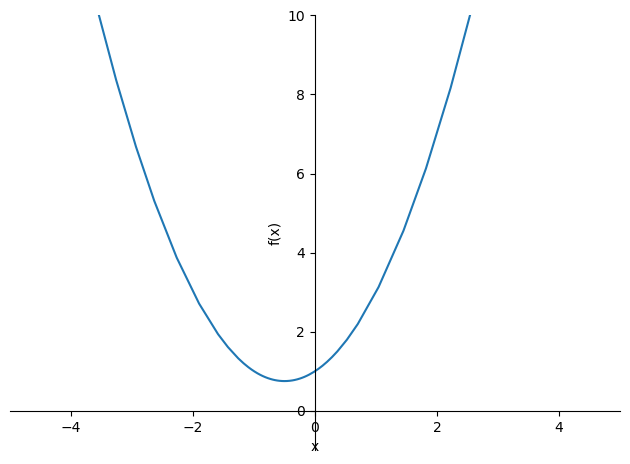
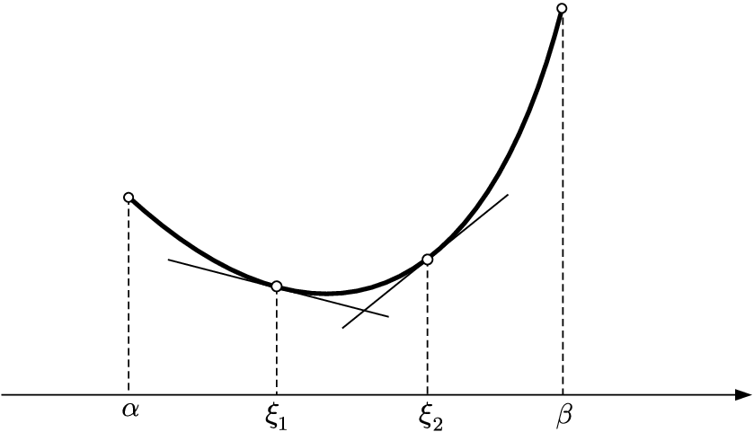
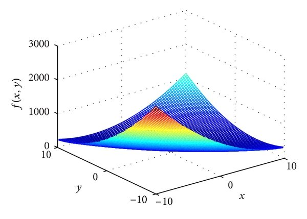
1. 볼록함수(Convex Function)
- 어떤 지점에서 시작하더라도 최적값(손실함수가 최소로 하는 점)에 도달할 수 있음
- 1-D Convex Function(1차원 볼록함수)
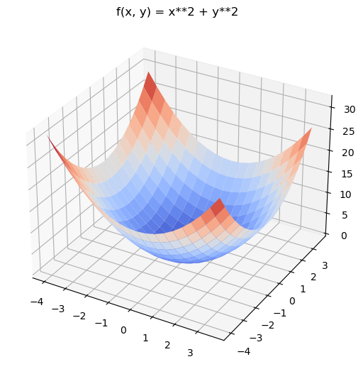
- 2-D Convex Function(2차원 볼록함수)
2. 비볼록함수(Non-Convex Function)
- 비볼록함수는 시작점의 위치에 따라 다른 최적값에 도달할 수 있음
- 1-D Non-Convex Function

- 2-D Non-Convex Function

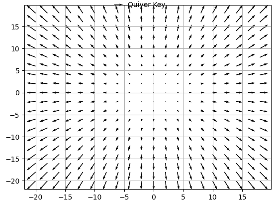
3. 미분과 기울기
- 스칼라를 벡터로 미분한 것
\(\frac{df(x)}{dx}=\underset{\triangle x \to 0}{lim}\frac{f(x+\triangle x)-f(x)}{\triangle x}\)

- \(\triangledown f(x)=\left ( \frac{\partial f}{\partial x_{1}}, \frac{\partial f}{\partial x_{2}}, \cdots, \frac{\partial f}{\partial x_{N}} \right )\)
- 변화가 있는 지점에서는 미분값이 존재하고, 변화가 없는 지점은 미분값이 0
- 미분값이 클수록 변화량이 크다는 의미
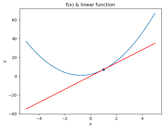
4. 경사하강법의 과정
- 경사하강법은 한 스텝마다의 미분값에 따라 이동하는 방향을 결정
- \(f(x)\)의 값이 변하지 않을 때까지 반복
$$ x_{n}=x_{n-1}-\eta \frac{\partial f}{\partial x} $$
- \(\eta\): 학습률(learning rate)
- 즉, 미분값이 0인 지점을 찾는 방법

- 2-D 경사하강법

5. 경사하강법 구현
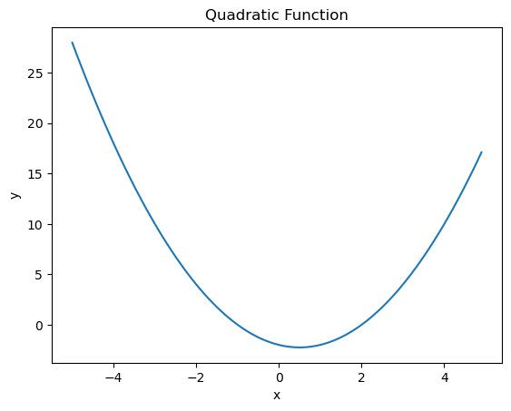
- \(f_{1}(x)=x^{2}
# 손실함수
def f1(x):
    return x**2

# 손실함수를 미분한 식
def df_dx1(x):
    return 2*x

# 경사하강법 구현
def gradient_descent(f, df_dx, init_x, learning_rate = 0.01, step_num = 100):
    x = init_x
    x_log, y_log = [x], [f(x)]
    for i in range(step_num):
        grad = df_dx(x)
        # 학습률에 미분한 기울기를 곱한 값만큼 x값을 변화시켜 최적값에 도달
        x -= learning_rate * grad

        x_log.append(x)
        y_log.append(f(x))

    return x_log, y_log
# 시각화
import matplotlib.pyplot as plt
import numpy as np
x_init = 5
x_log, y_log = gradient_descent(f1, df_dx1, init_x = x_init)
plt.scatter(x_log, y_log, color = 'red')
x = np.arange(-5, 5, 0.01)
plt.plot(x, f1(x))
plt.grid()
plt.show()
- 비볼록함수에서의 경사하강법
# 손실함수
def f2(x):
    return 0.01*x**4 - 0.3*x**3 - 1.0*x + 10.0

# 손실함수를 미분한 식
def df_dx2(x):
    return 0.04*x**3 - 0.9*x**2 - 1.0

# 시각화
x_init = 2
x_log, y_log = gradient_descent(f2, df_dx2, init_x = x_init)
plt.scatter(x_log, y_log, color = 'red')

x = np.arange(-5, 30, 0.01)
plt.plot(x, f2(x))
plt.xlim(-5, 30)
plt.grid()
plt.show()
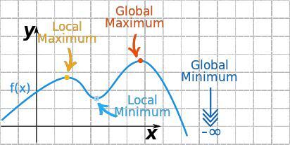
6. 전역최적값 vs 지역최적값
- 초기값이 어디냐에 따라 전체 함수의 최솟값이 될 수도 있고, 지역적으로 최솟값일 수도 있음
- \(f_{3}(x)=xsin(x^{2})+1\) 그래프
# 손실함수
def f3(x):
    return x*np.sin(x**2) + 1

# 손실함수를 미분한 식
def df_dx3(x):
    return np.sin(x**2) + x*np.cos(x**2)*2*x

# 시각화
x_init1 = -0.5
x_log1, y_log1 = gradient_descent(f3, df_dx3, init_x = x_init1)
plt.scatter(x_log1, y_log1, color = 'red')

x_init1 = -0.5
x_log1, y_log1 = gradient_descent(f3, df_dx3, init_x = x_init1)
plt.scatter(x_log1, y_log1, color = 'red')

x_init2 = 1.5
x_log2, y_log2 = gradient_descent(f3, df_dx3, init_x = x_init2)
plt.scatter(x_log2, y_log2, color = 'blue')

x = np.arange(-3, 3, 0.01)
plt.plot(x, f3(x), '--')

plt.scatter(x_init1, f3(x_init1), color = 'red')
plt.text(x_init1 - 1.0, f3(x_init1) + 0.3, "x_init1 ({})".format(x_init1), fontdict = {'size': 13})
plt.scatter(x_init2, f3(x_init2), color = 'blue')
plt.text(x_init2 - 0.7, f3(x_init2) + 0.4, "x_init2 ({})".format(x_init2), fontdict = {'size': 13})

plt.grid()
plt.show()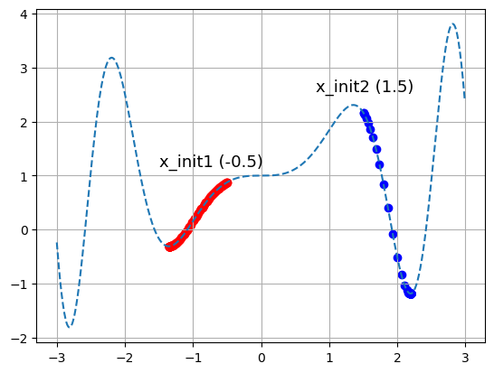
- 위의 그래프에서
- '전역최적값'은 x가 -3보다 조금 큰 부분
- x가 -0.5에서 시작했을 때 x가 찾아간 '지역최적값'은 -1보다 조금 작은 부분
- x가 1.5에서 시작했을 때 x가 찾아간 '지역최적값'은 2보다 조금 부분
7. 경사하강법 구현(2)
- 경사하강을 진행하는 도중, 최솟값에 이르면 경사하강법을 종료하는 코드
def gradient_descent2(f ,df_dx, init_x, learning_rate = 0.01, step_num = 100):
    eps = 1e-5
    count = 0

    old_x = init_x
    min_x = old_x
    min_y = f(min_x)

    x_log, y_log = [min_x], [min_y]
    for i in range(step_num):
        grad = df_dx(old_x)
        new_x = old_x - learning_rate * grad
        new_y = f(new_x)

        if min_y > new_y:
            min_x = new_x
            min_y = new_y

        if np.abs(old_x - new_x) < eps:
            break

        x_log.append(old_x)
        y_log.append(new_y)

        old_x = new_x
        count += 1

return x_log, y_log, count- \(f_{3}(x)=xsin(x^{2})+1\) 그래프
# 시각화
x_init1 = -2.2
x_log1, y_log1, count1 = gradient_descent2(f3, df_dx3, init_x = x_init1)
plt.scatter(x_log1, y_log1, color = 'red')
print("count:", count1)

x_init2 = -0.5
x_log2, y_log2, count2 = gradient_descent2(f3, df_dx3, init_x = x_init2)
plt.scatter(x_log2, y_log2, color = 'blue')
print("count:", count2)

x_init3 = 1.5
x_log3, y_log3, count3 = gradient_descent2(f3, df_dx3, init_x = x_init3)
plt.scatter(x_log3, y_log3, color = 'green')
print("count:", count3)

x = np.arange(-3, 3, 0.01)
plt.plot(x, f3(x), '--')

plt.scatter(x_init1, f3(x_init1), color = 'red')
plt.text(x_init1 + 0.2, f3(x_init1) + 0.2, "x_init1 ({})".format(x_init1), fontdict = {'size': 13})
plt.scatter(x_init2, f3(x_init2), color = 'blue')
plt.text(x_init2 + 0.1, f3(x_init2) - 0.3, "x_init2 ({})".format(x_init2), fontdict = {'size': 13})
plt.scatter(x_init3, f3(x_init3), color = 'green')
plt.text(x_init3 - 1.0, f3(x_init3) + 0.3, "x_init3 ({})".format(x_init3), fontdict = {'size': 13})

plt.grid()
plt.show()

# 출력 결과
count: 17
count: 100
count: 28
8. 학습률(Learning Rate)
- 학습률 값은 적절히 지정해야 함
- 너무 크면 발산, 너무작으면 학습이 잘 되지 않음

# learning rate가 굉장히 큰 경우(learning_rate = 1.05)
x_init = 10
x_log, y_log, _ = gradient_descent2(f1, df_dx1, init_x = x_init, learning_rate = 1.05)
plt.plot(x_log, y_log, color = 'red')

plt.scatter(x_init, f1(x_init), color = 'green')
plt.text(x_init - 2.2, f1(x_init) - 2, "x_init ({})".format(x_init), fontdict = {'size': 10})
x = np.arange(-50, 30, 0.01)
plt.plot(x, f1(x), '--')
plt.grid()
plt.show()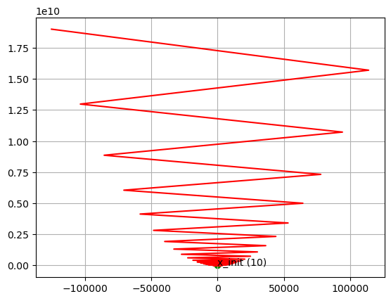
- 학습률별 경사하강법
lr_list = [0.001, 0.01, 0.1, 1.01]

init_x = 30.0
x = np.arange(-30, 50, 0.01)
fig = plt.figure(figsize = (12,10))

for i, lr in enumerate(lr_list):
    x_log, y_log, count = gradient_descent2(f1, df_dx1, init_x = x_init, learning_rate = lr)
    ax = fig.add_subplot(2, 2, i+1)
    ax.scatter(init_x, f1(init_x), color = 'green')
    ax.plot(x_log, y_log, color = 'red', linewidth = '4')
    ax.plot(x, f1(x), '--')
    ax.grid()
    ax.title.set_text('learning_rate = {}'.format(str(lr)))
    print("init value = {}, count = {}".format(str(lr), str(count)))

plt.show()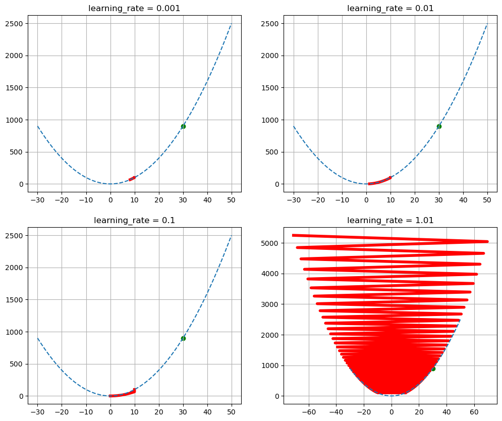
9. 안장점(Saddle Point)
- 기울기가 0이지만 극값이 되지 않음
- 경사하강법은 안장점에서 벗어나지 못함

- \(f_{2}(x)=0.01x^{4}-0.3x^{3}-1.0x+10.0\) 그래프로 확인하기
- 첫번째 시작점
- count가 100, 즉 step_num(반복횟수)만큼 루프를 돌았음에도 손실함수의 값이 10 언저리에서 멈춤, 변화 x
- 이는 학습률 조절 또는 다른 초기값 설정을 통해 수정해야 함
x_init1 = -10.0
x_log1, y_log1, count1 = gradient_descent2(f2, df_dx2, init_x = x_init1)
plt.scatter(x_log1, y_log1, color = 'red')
print("count:", count1)

x_init2 = 5.0
x_log2, y_log2, count2 = gradient_descent2(f2, df_dx2, init_x = x_init2)
plt.scatter(x_log2, y_log2, color = 'blue')
print("count:", count2)

x_init3 = 33.0
x_log3, y_log3, count3 = gradient_descent2(f2, df_dx2, init_x = x_init3)
plt.scatter(x_log3, y_log3, color = 'green')
print("count:", count3)

x = np.arange(-15, 35, 0.01)
plt.plot(x, f2(x), '--')

plt.scatter(x_init1, f2(x_init1), color = 'red')
plt.text(x_init1 + 2, f2(x_init1), "x_init1 ({})".format(x_init1), fontdict = {'size': 13})
plt.scatter(x_init2, f2(x_init2), color = 'blue')
plt.text(x_init2 + 2, f2(x_init2) + 53, "x_init2 ({})".format(x_init2), fontdict = {'size': 13})
plt.scatter(x_init3, f2(x_init3), color = 'green')
plt.text(x_init3 - 18, f2(x_init3), "x_init3 ({})".format(x_init3), fontdict = {'size': 13})

plt.grid()
plt.show()

# 출력 결과
count: 100
count: 82
count: 50
- \(f_{3}(x)=xsin(x^{2})+1\) 그래프로 확인하기
x_init1 = -2.2
x_log1, y_log1, count1 = gradient_descent2(f3, df_dx3, init_x = x_init1)
plt.scatter(x_log1, y_log1, color = 'red')
print("count:", count1)

x_init2 = 1.2
x_log2, y_log2, count2 = gradient_descent2(f3, df_dx3, init_x = x_init2)
plt.scatter(x_log2, y_log2, color = 'blue')
print("count:", count2)

x = np.arange(-3, 3, 0.01)
plt.plot(x, f3(x), '--')

plt.scatter(x_init1, f3(x_init1), color = 'red')
plt.text(x_init1 + 0.2, f3(x_init1) + 0.2, "x_init1 ({})".format(x_init1), fontdict = {'size': 13})
plt.scatter(x_init2, f3(x_init2), color = 'blue')
plt.text(x_init2 - 1.0, f3(x_init2) + 0.3, "x_init2 ({})".format(x_init2), fontdict = {'size': 13})

plt.grid()
plt.show()

# 출력 결과
count: 17
count: 100
'Python > Deep Learning' 카테고리의 다른 글
| [딥러닝 기초] 오차역전파(Backpropagation) (0) | 2023.03.15 |
|---|---|
| [딥러닝 기초] 신경망 학습 (0) | 2023.03.14 |
| [딥러닝 기초] 모델 학습과 손실 함수 (1) | 2023.03.12 |
| [딥러닝 기초] 신경망 구조 (0) | 2023.03.09 |
| [딥러닝 기초] 신경망 데이터 표현 (0) | 2023.03.08 |