1. 순환 신경망(Recurrent Neural Network, RNN)
- 루프(loop)를 가진 신경망의 한 종류
- 시퀀스의 원소를 순회하면서 지금가지 처리한 정보를 상태(state)에 저장
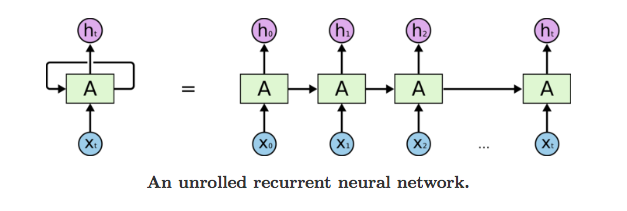
- 순환 신경망 레이어(RNN Layer)
- 입력: (timesteps, input_features)
- 출력: (timesteps, output_features)
# numpy로 RNN 구조 표현
import numpy as np

timesteps = 100
input_features = 32
output_features = 64

inputs = np.random.random((timesteps, input_features))

state_t = np.zeros((output_features, ))

W = np.random.random((output_features, input_features))
U = np.random.random((output_features, output_features))
b = np.random.random((output_features, ))

sucessive_outputs = []

for input_t in inputs:
    output_t = np.tanh(np.dot(W, input_t) + np.dot(U, state_t) + b)
    sucessive_outputs.append(output_t)
    state_t = output_t

final_output_sequence = np.stack(sucessive_outputs, axis = 0)
- 케라스의 순환층
- SimpleRNN layer
- 입력: (batch_size, timesteps, input_features)
- 출력
- return_sequences로 결정할 수 있음
- 3D 텐서
- timesteps의 출력을 모든 전체 sequences를 반환
- (batch_size, timesteps, output_features)
- 2D 텐서
- 입력 sequence에 대한 마지막 출력만 반환
- (batch_size, output_features)
from tensorflow.keras.layers import SimpleRNN, Embedding
from tensorflow.keras.models import Sequential

model = Sequential()
model.add(Embedding(10000, 32))
model.add(SimpleRNN(32))  # SimpleRNN 안에 return_sequences = True옵션을 추가하면 전체 sequences를 return시켜줌
model.summary()

# 출력 결과
Model: "sequential"
_________________________________________________________________
 Layer (type)                Output Shape              Param #
=================================================================
 embedding (Embedding)       (None, None, 32)          320000

 simple_rnn (SimpleRNN)      (None, 32)                2080

=================================================================
Total params: 322,080
Trainable params: 322,080
Non-trainable params: 0
_________________________________________________________________- 네트워크의 표현력을 증가시키기 위해 여러 개의 순환층을 차례대로 쌓는 것이 유용할 때가 있음
- 이런 설정에서는 중간층들이 전체 출력 sequences를 반환하도록 설정
model = Sequential()
model.add(Embedding(10000, 32))
model.add(SimpleRNN(32, return_sequences = True))
model.add(SimpleRNN(32, return_sequences = True))
model.add(SimpleRNN(32, return_sequences = True))
model.add(SimpleRNN(32))
model.summary()

# 출력 결과
Model: "sequential_2"
_________________________________________________________________
 Layer (type)                Output Shape              Param #
=================================================================
 embedding_2 (Embedding)     (None, None, 32)          320000

 simple_rnn_2 (SimpleRNN)    (None, None, 32)          2080

 simple_rnn_3 (SimpleRNN)    (None, None, 32)          2080

 simple_rnn_4 (SimpleRNN)    (None, None, 32)          2080

 simple_rnn_5 (SimpleRNN)    (None, 32)                2080

=================================================================
Total params: 328,320
Trainable params: 328,320
Non-trainable params: 0
_________________________________________________________________
- LMDB 데이터 적용
- 데이터 로드
from tensorflow.keras.datasets import imdb
from tensorflow.keras.preprocessing import sequence

num_words = 10000
max_len = 500
batch_size = 32

(input_train, y_train), (input_test, y_test) = imdb.load_data(num_words = num_words)
print(len(input_train))  # 25000
print(len(input_test))   # 25000

input_train = sequence.pad_sequences(input_train, maxlen = max_len)
input_test = sequence.pad_sequences(input_test, maxlen = max_len)
print(input_train.shape) # (25000, 500)
print(input_test.shape)  # (25000, 500)
- 모델 구성
from tensorflow.keras.layers import Dense

model = Sequential()

model.add(Embedding(num_words, 32))
model.add(SimpleRNN(32))
model.add(Dense(1, activation = 'sigmoid'))

model.compile(optimizer = 'rmsprop',
              loss = 'binary_crossentropy',
              metrics = ['acc'])

model.summary()

# 출력 결과
Model: "sequential_3"
_________________________________________________________________
 Layer (type)                Output Shape              Param #
=================================================================
 embedding_3 (Embedding)     (None, None, 32)          320000

 simple_rnn_6 (SimpleRNN)    (None, 32)                2080

 dense (Dense)               (None, 1)                 33

=================================================================
Total params: 322,113
Trainable params: 322,113
Non-trainable params: 0
_________________________________________________________________
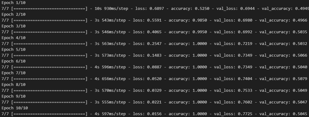
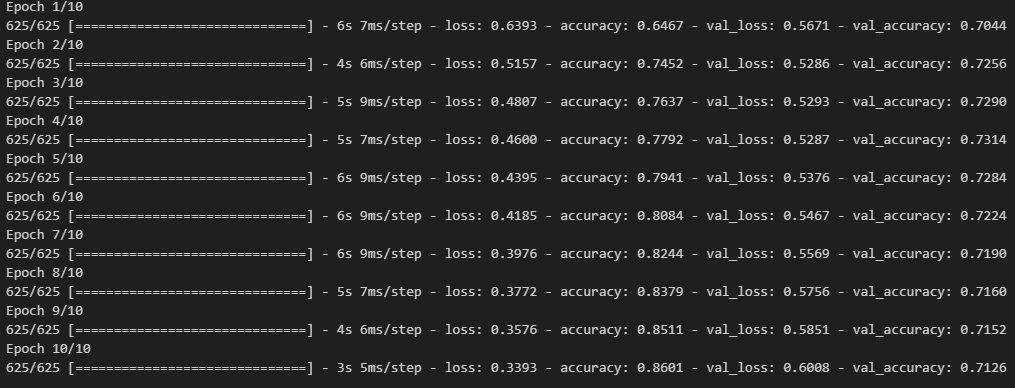
- 모델 학습
history = model.fit(input_train, y_train,
                    epochs = 10,
                    batch_size = 128,
                    validation_split = 0.2)
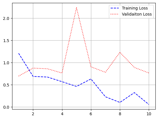
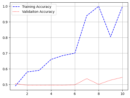
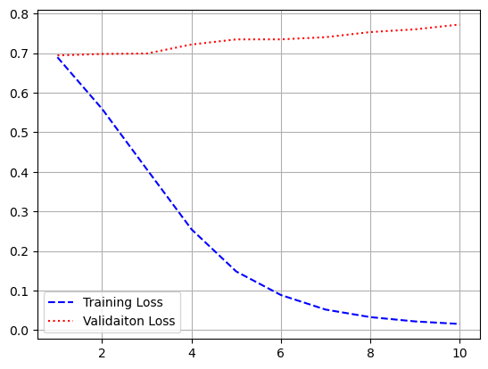
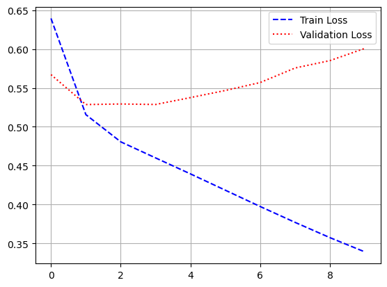
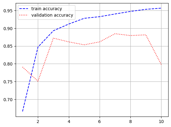
- 시각화
import matplotlib.pyplot as plt
loss = history.history['loss']
val_loss = history.history['val_loss']
acc = history.history['acc']
val_acc = history.history['val_acc']
epochs = range(1, len(loss) + 1)
plt.plot(epochs, loss, 'b--', label = 'train loss')
plt.plot(epochs, val_loss, 'r:', label = 'validation loss')
plt.grid()
plt.legend()
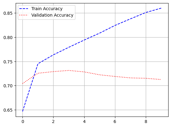
plt.figure()
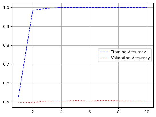
plt.plot(epochs, acc, 'b--', label = 'train accuracy')
plt.plot(epochs, val_acc, 'r:', label = 'validation accuracy')
plt.grid()
plt.legend()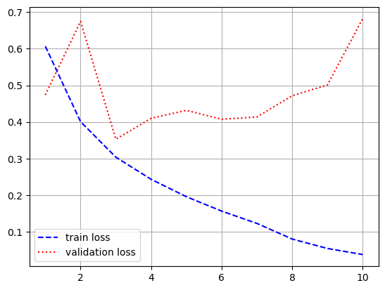
model.evaluate(input_test, y_test)

# 출력 결과
loss: 0.6755 - acc: 0.7756
[0.6754735112190247, 0.7755600214004517]- 전체 sequences가 아니라 순서대로 500개의 단어만 입력했기 때문에 성능이 낮게 나옴
- simpleRNN은 긴 sequence를 처리하는데 적합하지 않음
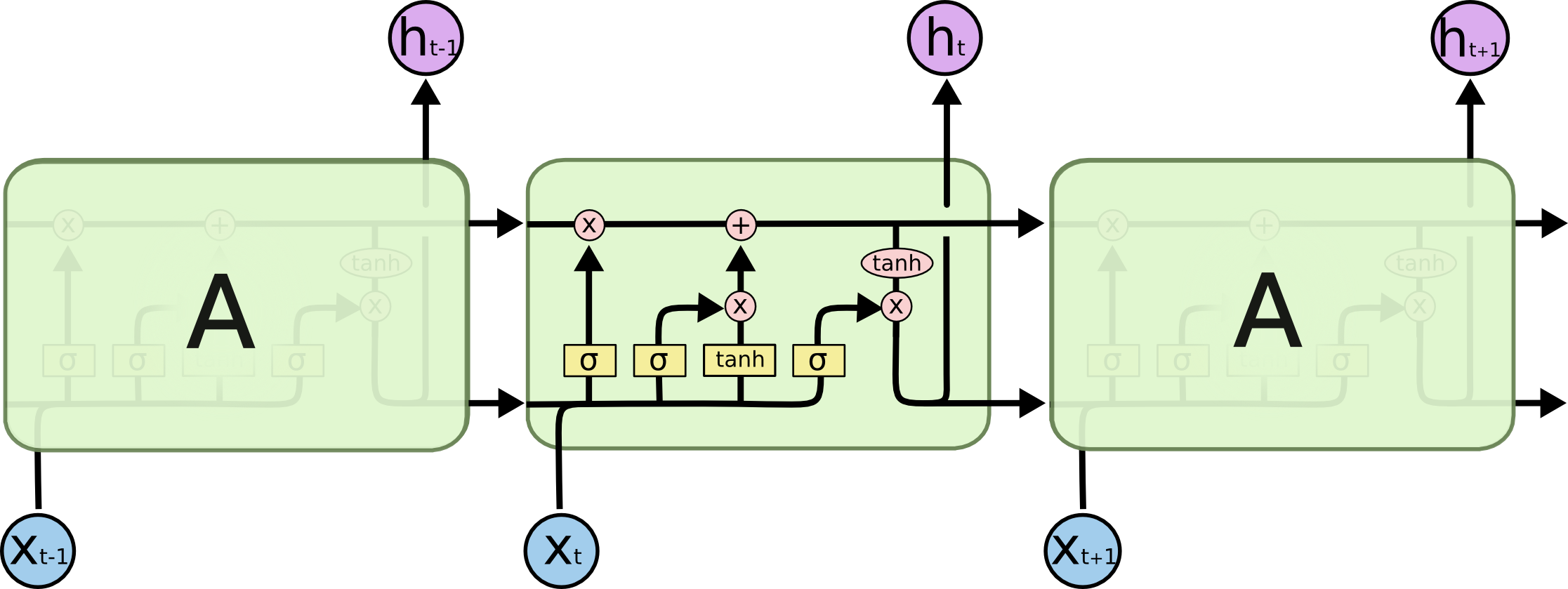
2. LSTM과 GRU 레이어
- Simple RNN은 실전에 사용하기엔 너무 단순
- SimpleRNN은 이론적으로 시간 t에서 이전의 모든 timesteps의 정보를 유지할 수 있지만, 실제로는 긴 시간에 걸친 의존성은 학습할 수 없음
- 그레디언트 소실 문제(vanishing gradient problem)
- 이를 방지하기 위해 LSTM, GRU 같은 레이어 등장
- LSTM(Long-Short-Term Memory)
- 장단기 메모리 알고리즘
- 나중을 위해 정보를 저장함으로써 오래된 시그널이 점차 소실되는 것을 막아줌
- 예제 1) Reyters
- IMDB와 유사한 데이터셋(텍스트 데이터)
- 46개의 상호 배타적인 토픽으로 이루어진 데이터셋
- 다중 분류 문제
- 데이터셋 로드
from tensorflow.keras.datasets import reuters

num_words = 10000
(x_train, y_train), (x_test, y_test) = reuters.load_data(num_words = num_words)

print(x_train.shape) # (8982,)
print(y_train.shape) # (8982,)
print(x_test.shape)  # (2246,)
print(y_test.shape)  # (2246,)
- 데이터 전처리 및 확인
from tensorflow.keras.preprocessing.sequence import pad_sequences

max_len = 500

pad_x_train = pad_sequences(x_train, maxlen = max_len)
pad_x_test = pad_sequences(x_test, maxlen = max_len)

print(len(pad_x_train[0]))  # 500

pad_x_train[0]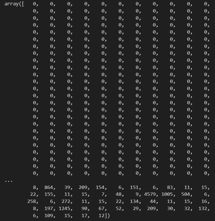
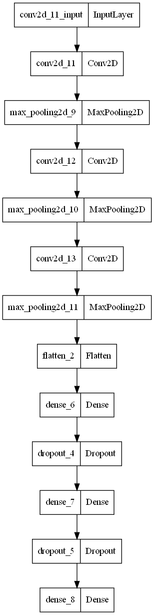
- 모델 구성
- LSTM 레이어도 SimpleRNN과 같이 return_sequences 인자 사용 가능
from tensorflow.keras.models import Sequential
from tensorflow.keras.layers import LSTM, Dense, Embedding

model = Sequential()
model.add(Embedding(input_dim = num_words, output_dim = 64))
model.add(LSTM(64, return_sequences = True))
model.add(LSTM(32))
model.add(Dense(46, activation = 'softmax'))

model.compile(optimizer = 'adam',
              loss = 'sparse_categorical_crossentropy',
              metrics = ['acc'])
model.summary()

# 출력 결과
Model: "sequential_1"
_________________________________________________________________
 Layer (type)                Output Shape              Param #
=================================================================
 embedding_1 (Embedding)     (None, None, 64)          640000

 lstm (LSTM)                 (None, None, 64)          33024

 lstm_1 (LSTM)               (None, 32)                12416

 dense (Dense)               (None, 46)                1518

=================================================================
Total params: 686,958
Trainable params: 686,958
Non-trainable params: 0
_________________________________________________________________
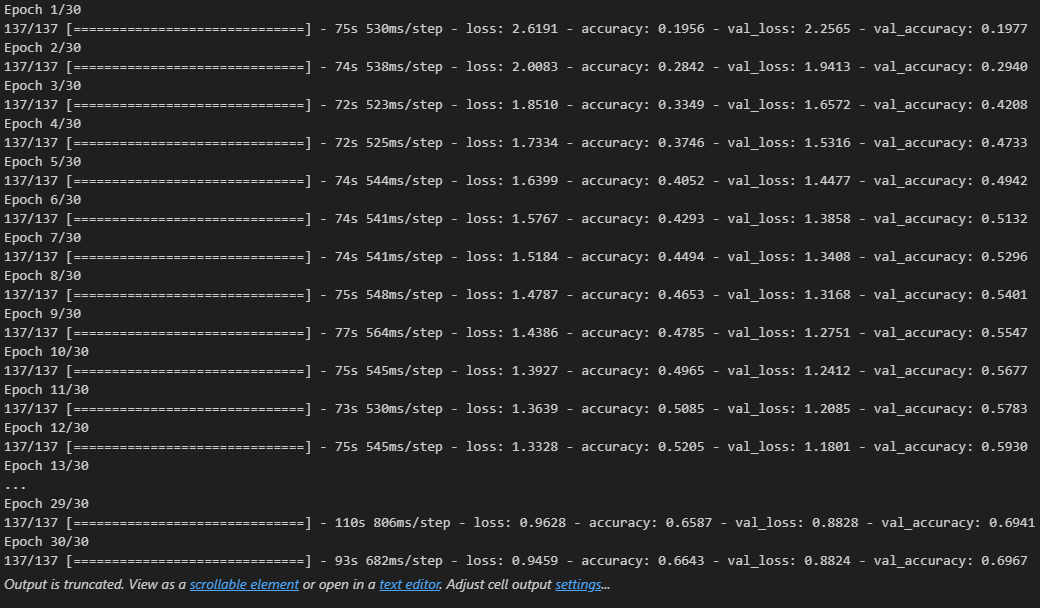
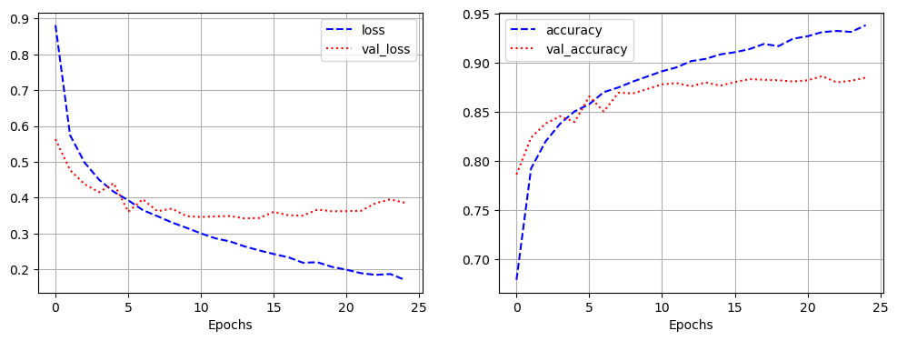
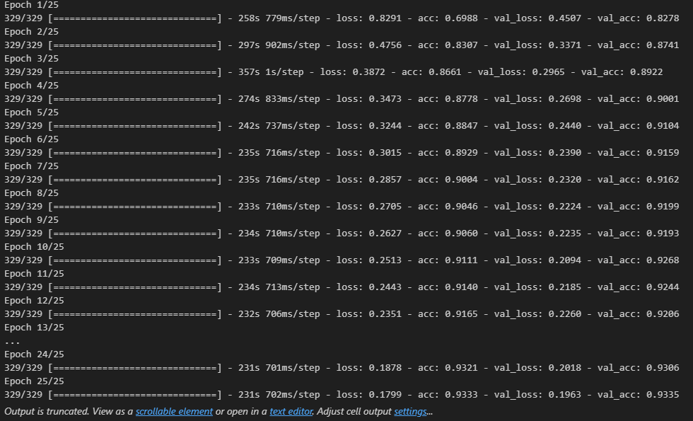
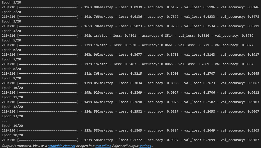
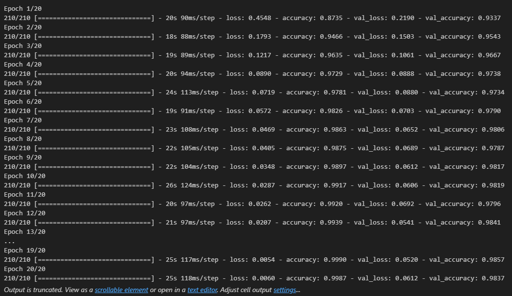
- 모델 학습
history = model.fit(pad_x_train, y_train,
                    epochs = 20,
                    batch_size = 32,
                    validation_split = 0.2)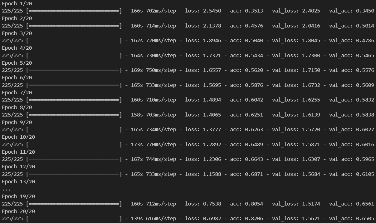
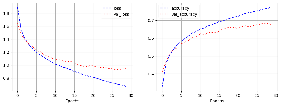
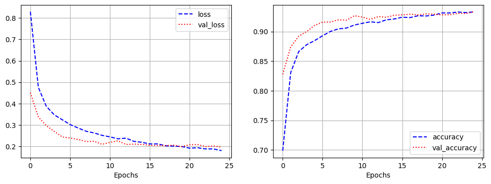
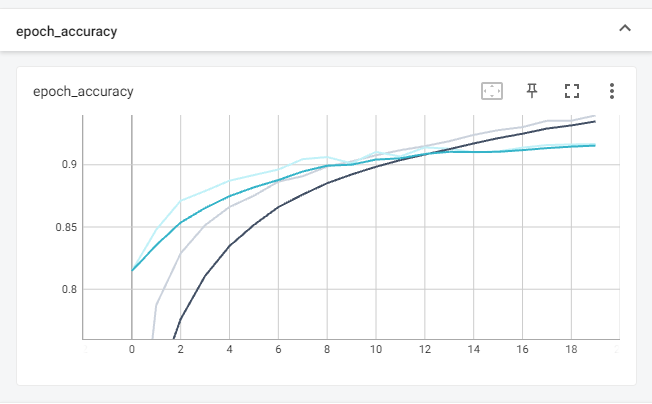
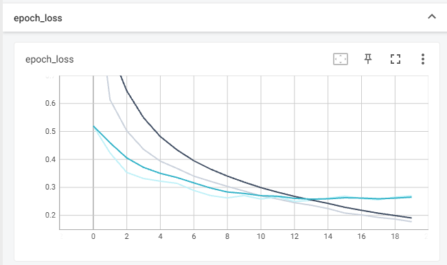
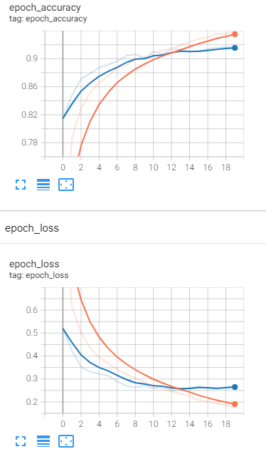
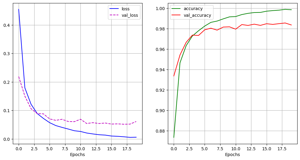
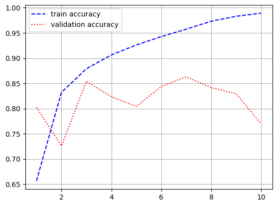
- 시각화
import matplotlib.pyplot as plt

loss = history.history['loss']
val_loss = history.history['val_loss']
acc = history.history['acc']
val_acc = history.history['val_acc']

epochs = range(1, len(loss) + 1)

plt.plot(epochs, loss, 'b--', label = 'train loss')
plt.plot(epochs, val_loss, 'r:', label = 'validation loss')
plt.grid()
plt.legend()

plt.figure()
plt.plot(epochs, acc, 'b--', label = 'train accuracy')
plt.plot(epochs, val_acc, 'r:', label = 'validation accuracy')
plt.grid()
plt.legend()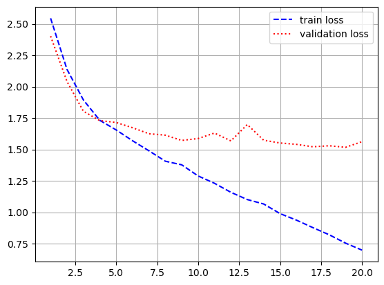
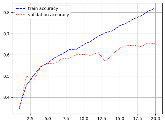
- 모델 평가
model.evaluate(pad_x_test, y_test)

# 출력 결과
loss: 1.6927 - acc: 0.6336
[1.692732810974121, 0.6335707902908325]
- 예제 2) IMDB 데이터셋
- 데이터 로드
from tensorflow.keras.datasets import imdb
from tensorflow.kears.preprocessing.sequence import pad_sequences

num_words = 10000
max_len = 500
batch_size = 32

(x_train, y_train), (x_test, y_test) = imdb.load_data(num_words = num_words)

pad_x_train = sequence.pad_sequences(x_train, maxlen = max_len)
pad_x_test = sequence.pad_sequences(x_test, maxlen = max_len)
- 모델 구성
from tensorflow.keras.models import Sequential
from tensorflow.keras.layers import Dense, LSTM, Embedding

model = Sequential()
model.add(Embedding(num_words, 32))
model.add(LSTM(32))
model.add(Dense(1, activation = 'sigmoid'))

model.compile(optimizer = 'rmsprop',
              loss = 'binary_crossentropy',
              metrics = ['acc'])
model.summray()

# 출력 결과
Model: "sequential_3"
_________________________________________________________________
 Layer (type)                Output Shape              Param #
=================================================================
 embedding_3 (Embedding)     (None, None, 32)          320000

 lstm_3 (LSTM)               (None, 32)                8320

 dense_2 (Dense)             (None, 1)                 33

=================================================================
Total params: 328,353
Trainable params: 328,353
Non-trainable params: 0
_________________________________________________________________
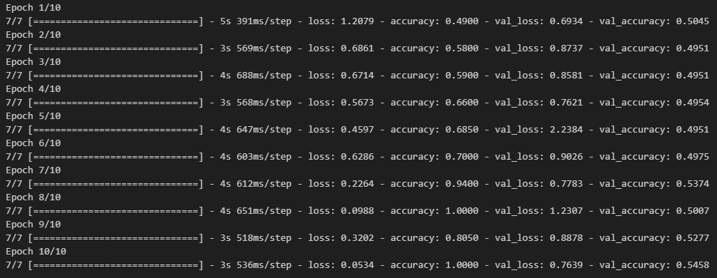
- 모델 학습
history = model.fit(pad_x_train, y_train,
                    epochs = 10,
                    batch_size = 128,
                    validation_split = 0.2)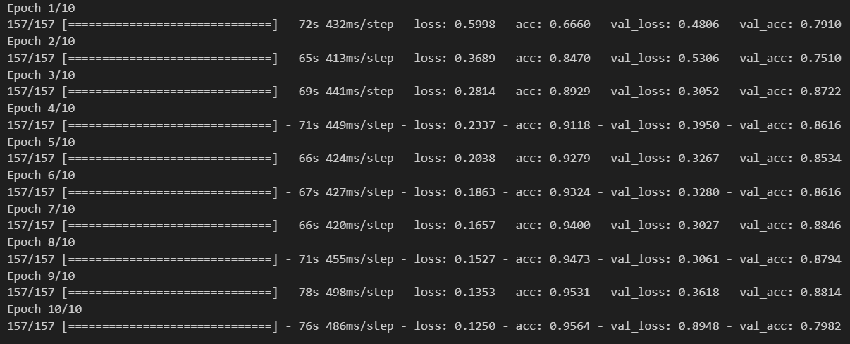
- 시각화
import matplotlib.pyplot as plt

loss = history.history['loss']
val_loss = history.history['val_loss']
acc = history.history['acc']
val_acc = history.history['val_acc']

epochs = range(1, len(loss) + 1)

plt.plot(epochs, loss, 'b--', label = 'train loss')
plt.plot(epochs, val_loss, 'r:', label = 'validation loss')
plt.grid()
plt.legend()

plt.figure()
plt.plot(epochs, acc, 'b--', label = 'train accuracy')
plt.plot(epochs, val_acc, 'r:', label = 'validation accuracy')
plt.grid()
plt.legend()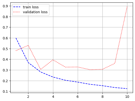
- 모델 평가
model.evaluate(pad_x_test, y_test)

# 출력 결과
loss: 0.9135 - acc: 0.7898
[0.9135046601295471, 0.7898399829864502]- LSTM 쓰기전, SimpleRNN을 썻을 때 loss가 0.6755, acc가 0.7756으로 나온 것에 비해 좋은 결과가 나옴
3. Cosine 함수를 이용한 순환 신경망
# 코사인 시계열 데이터
import numpy as np

np.random.seed(111)
time = np.arange(30 * 12 + 1)
month_time = (time % 30) / 30
time_series = 20 * np.where(month_time < 0.5,
                            np.cos(2 * np.pi * month_time),
                            np.cos(2 * np.pi * month_time) + np.random.random(361))
plt.figure(figsize = (15, 8))
plt.xlabel('Time')
plt.ylabel('Value')
plt.plot(np.arange(0, 30 * 11 + 1),
         time_series[:30 * 11 + 1],
         color = 'blue', alpha = 0.6, label = 'Train Data')
plt.plot(np.arange(30 * 11, 30 * 12 + 1),
         time_series[30 * 11:],
         color = 'orange', label = 'Test Data')
plt.show()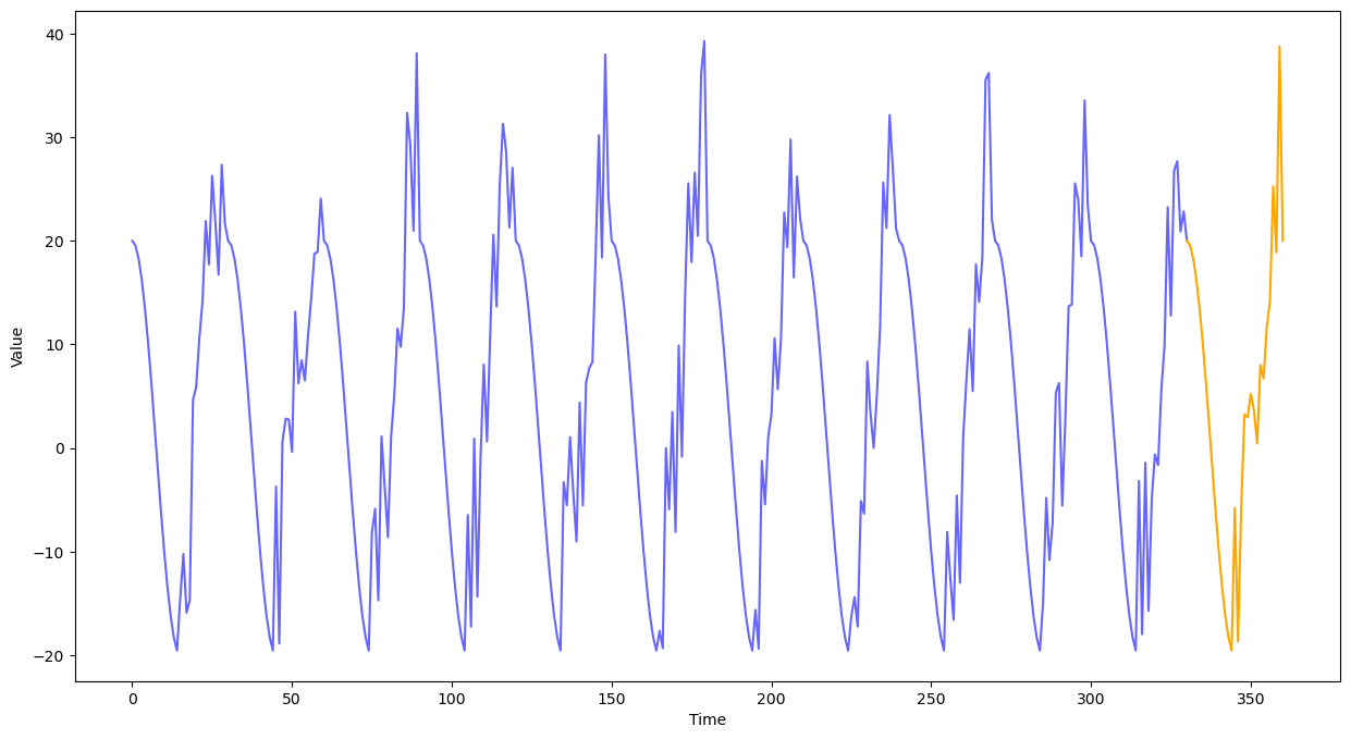
- 데이터 전처리
def make_data(time_series, n):
    x_train_full, y_train_full = list(), list()

    for i in range(len(time_series)):
        x = time_series[i:(i + n)]
        if (i + n) < len(time_series):
            x_train_full.append(x)
            y_train_full.append(time_series[i + n])
        else:
            break

    x_train_full, y_train_full = np.array(x_train_full), np.array(y_train_full)

    return x_train_full, y_train_full

n = 10
x_train_full, y_train_full = make_data(time_series, n)

print(x_train_full.shape) # (351, 10)
print(y_train_full.shape) # (351,)


# 뒤에 1씩 추가
x_train_full = x_train_full.reshape(-1, n, 1)
y_train_full = y_train_full.reshape(-1, n, 1)

print(x_train_full.shape) # (351, 10, 1)
print(y_train_full.shape) # (351, 1)
- 테스트 데이터셋 생성
x_train_full = x_train_full.reshape(-1, n, 1)
y_train_full = y_train_full.reshape(-1, n, 1)

print(x_train_full.shape)
print(y_train_full.shape)


# train 데이터와 test 데이터 분리
x_train = x_train_full[:30 * 11]
y_train = y_train_full[:30 * 11]

x_test = x_train_full[30 * 11:]
y_test = y_train_full[30 * 11:]

print(x_train.shape) # (330, 10, 1)
print(y_train.shape) # (330, 1)
print(x_test.shape)  # (21, 10, 1)
print(y_test.shape)  # (21, 10, 1)
- 데이터 확인
sample_series = np.arange(100)
a, b = make_data(sample_series, 10)

print(a[0])  # [0 1 2 3 4 5 6 7 8 9]
print(b[0])  # 10
- 모델 구성
from tensorflow.keras.layers import SimpleRNN, Flatten, Dense
from tensorflow.keras.models import Sequential

def build_model(n):
    model = Sequential()

    model.add(SimpleRNN(units = 32, activation = 'tanh', input_shape = (n, 1)))
    model.add(Dense(1))

    model.compile(optimizer = 'adam',
                  loss = 'mse')
    return model

model = build_model(10)
model.summary()

# 출력 결과
Model: "sequential_4"
_________________________________________________________________
 Layer (type)                Output Shape              Param #
=================================================================
 simple_rnn (SimpleRNN)      (None, 32)                1088

 dense_3 (Dense)             (None, 1)                 33

=================================================================
Total params: 1,121
Trainable params: 1,121
Non-trainable params: 0
_________________________________________________________________
- 모델 학습
model.fit(x_train, y_train,
          epochs = 100, batch_size = 12)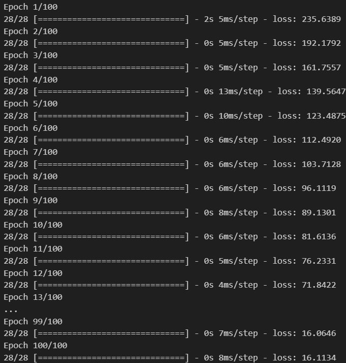
- 예측값 그려보기
prediction = model.predict(x_test)

pred_range = np.arange(len(y_train), len(y_train) + len(prediction))

plt.figure(figsize = (12, 5))
plt.xlabel('Time')
plt.ylabel('Value')
plt.plot(pred_range, y_test.flatten(), color = 'orange', label = 'Ground Truth')
plt.plot(pred_range, prediction.flatten(), color = 'blue', label = 'Prediction')
plt.legend()
plt.show()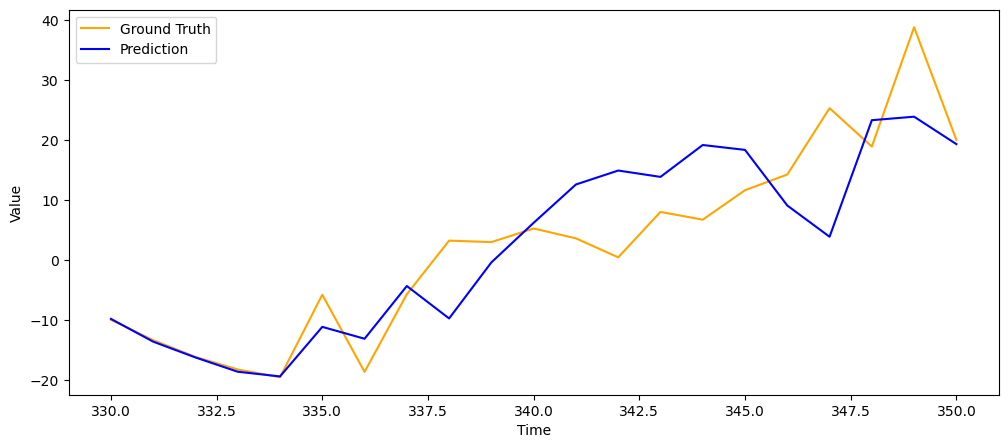
- 모델 재구성
- LSTM 사용
from tensorflow.keras.layers import LSTM

def build_model2(n):
    model = Sequential()

    model.add(LSTM(units = 64, return_sequences = True, input_shape = (n, 1)))
    model.add(LSTM(32))
    model.add(Dense(1))

    model.compile(optimizer = 'adam',
                  loss = 'mse')
    return model

model2 = build_model2(10)
model2.summary()

# 출력 결과
Model: "sequential_6"
_________________________________________________________________
 Layer (type)                Output Shape              Param #
=================================================================
 lstm_4 (LSTM)               (None, 10, 64)            16896

 lstm_5 (LSTM)               (None, 32)                12416

 dense_5 (Dense)             (None, 1)                 33

=================================================================
Total params: 29,345
Trainable params: 29,345
Non-trainable params: 0
_________________________________________________________________
- 모델 재학습 및 예측값 그려보기
model2.fit(x_train, y_train,
           epochs = 100, batch_size = 12)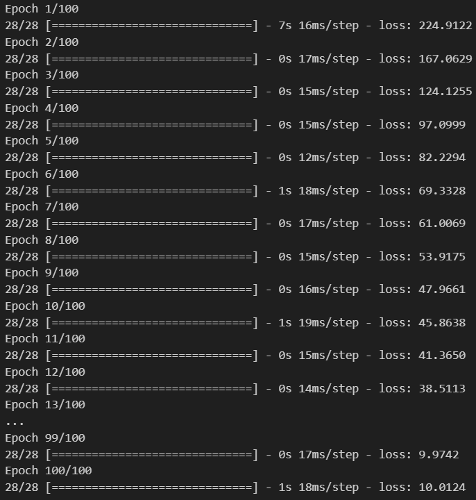
prediction_2 = model_2.predict(x_test)

pred_range = np.arange(len(y_train), len(y_train) + len(prediction_2))

plt.figure(figsize = (12, 5))
plt.xlabel('Time')
plt.ylabel('Value')
plt.plot(pred_range, y_test.flatten(), color = 'orange', label = 'Ground Truth')
plt.plot(pred_range, prediction.flatten(), color = 'r:', label = 'Model1 Prediction')
plt.plot(pred_range, prediction_2.flatten(), color = 'blue', label = 'Model2 Prediction')
plt.legend()
plt.show()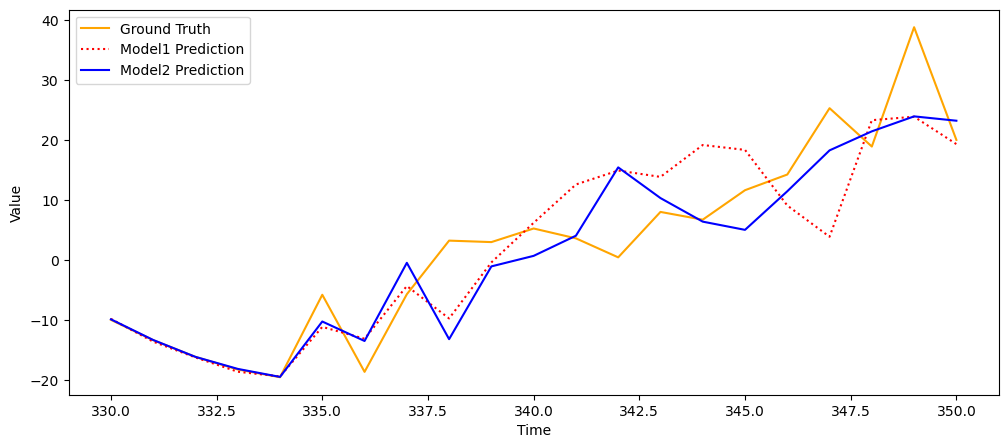
- 모델 재구성
- GRU 사용(LSTM보다 더 쉬운 구조)
from tensorflow.keras.layers import GRU

def build_model3(n):
    model = Sequential()

    model.add(GRU(units = 30, return_sequences = True, input_shape = (n, 1)))
    model.add(GRU(30))
    model.add(Dense(1))

    model.compile(optimizer = 'adam',
                  loss = 'mse')
    return model

model_3 = build_model3(10)
model_3.summary()

# 출력 결과
Model: "sequential_7"
_________________________________________________________________
 Layer (type)                Output Shape              Param #
=================================================================
 lstm_6 (LSTM)               (None, 10, 64)            16896

 lstm_7 (LSTM)               (None, 32)                12416

 dense_6 (Dense)             (None, 1)                 33

=================================================================
Total params: 29,345
Trainable params: 29,345
Non-trainable params: 0
_________________________________________________________________
- 모델 재학습 및 예측값 그려보기
model_3.fit(x_train, y_train,
           epochs = 100, batch_size = 12)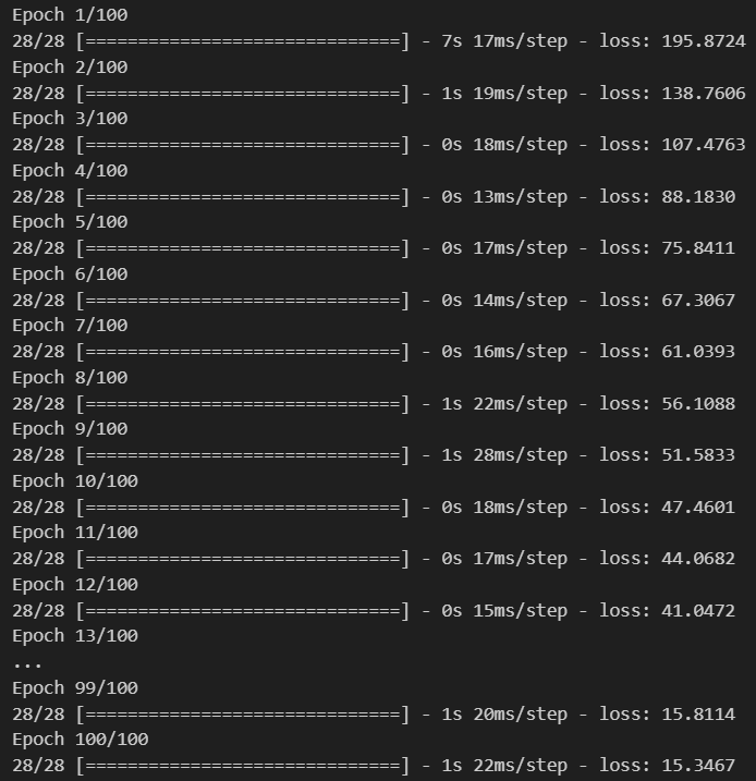
prediction_3 = model_3.predict(x_test)

pred_range = np.arange(len(y_train), len(y_train) + len(prediction_3))

plt.figure(figsize = (12, 5))
plt.xlabel('Time')
plt.ylabel('Value')
plt.plot(pred_range, y_test.flatten(), color = 'orange', label = 'Ground Truth')
plt.plot(pred_range, prediction.flatten(), color = 'r:', label = 'Model1 Prediction')
plt.plot(pred_range, prediction_2.flatten(), color = 'blue', label = 'Model2 Prediction')
plt.plot(pred_range, prediction_2.flatten(), color = 'blue', label = 'Model3 Prediction')
plt.legend()
plt.show()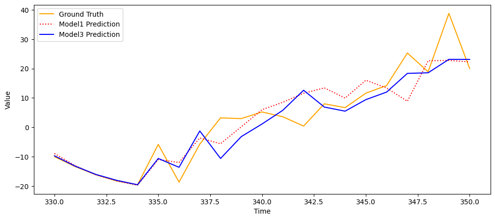
- Conv1D
- 텍스트 분류나 시계열 예측같은 간단한 문제, 오디오 생성, 기계 번역 등의 문제에서 좋은 성능
- timestep의 순서에 민감 X
- 2D Convolution
- 지역적 특징을 인식
- 2D Convolution
- 문맥을 인식
- Conv1D Layer
- 입력: (batch_size, timesteps, channels)
- 출력: (batch_size, timesteps, filters)
- 필터의 사이즈가 커져도 모델이 급격히 증가하지 않기 때문에 다양한 크기를 사용할 수 있음
- 데이터의 품질이 좋으면 굳이 크기를 달리하여 여러 개를 사용하지 않아도 될 수도 있음
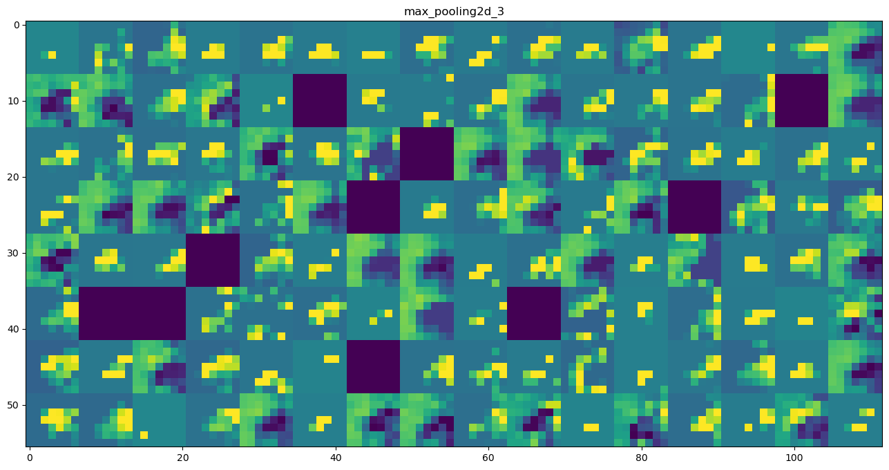
- MaxPooling1D Layer
- 다운 샘플링 효과
- 단지 1차원형태로 바뀐 것 뿐
- GlovalMaxPooling Layer
- 배치 차원을 제외하고 2차원 형태를 1차원 형태로 바꾸어주는 레이어
- Flatten layer로 대신 사용가능
- IMDB 데이터셋
- 데이터 로드 및 전처리
from tensorflow.keras.datasets import imdb
from tensorflow.keras.preprocessing.sequence import pad_sequences
from tensorflow.keras.models import Sequential
from tensorflow.keras.optimizers import RMSprop
from tensorflow.keras.layers import Dense, Embedding, Conv1D, MaxPooling1D, GlobalMaxPooling1D

num_words = 10000
max_len = 500
batch_size = 32

(input_train, y_train), (input_test, y_test) = imdb.load_data(num_words = num_words)

print(len(input_train))  # 25000
print(len(input_test))   # 25000

pad_x_train = pad_sequences(input_train, maxlen = max_len)
pad_x_test = pad_sequences(input_test, maxlen = max_len)

print(pad_x_train.shape) # (25000, 500)
print(pad_x_test.shape)  # (25000, 500)
-모델 구성
def build_model():
    model = Sequential()

    model.add(Embedding(input_dim = num_words, output_dim = 32,
                        input_length = max_len))
    model.add(Conv1D(32, 7, activation = 'relu'))
    model.add(MaxPooling1D(7))
    model.add(Conv1D(32, 5, activation = 'relu'))
    model.add(MaxPooling1D(5))
    model.add(GlobalMaxPooling1D())
    model.add(Dense(1, activation = 'sigmoid'))

    model.compile(optimizer = RMSprop(learning_rate = 1e-4),
                  loss ='binary_crossentropy',
                  metrics = ['accuracy'])

    return model

model = build_model()
model.summary()

# 출력 결과
Model: "sequential_13"
_________________________________________________________________
 Layer (type)                Output Shape              Param #
=================================================================
 embedding_5 (Embedding)     (None, 500, 32)           320000

 conv1d_2 (Conv1D)           (None, 494, 32)           7200

 max_pooling1d_2 (MaxPooling  (None, 70, 32)           0
 1D)

 conv1d_3 (Conv1D)           (None, 66, 32)            5152

 max_pooling1d_3 (MaxPooling  (None, 13, 32)           0
 1D)

 global_max_pooling1d_1 (Glo  (None, 32)               0
 balMaxPooling1D)

 dense_12 (Dense)            (None, 1)                 33

=================================================================
Total params: 332,385
Trainable params: 332,385
Non-trainable params: 0
_________________________________________________________________
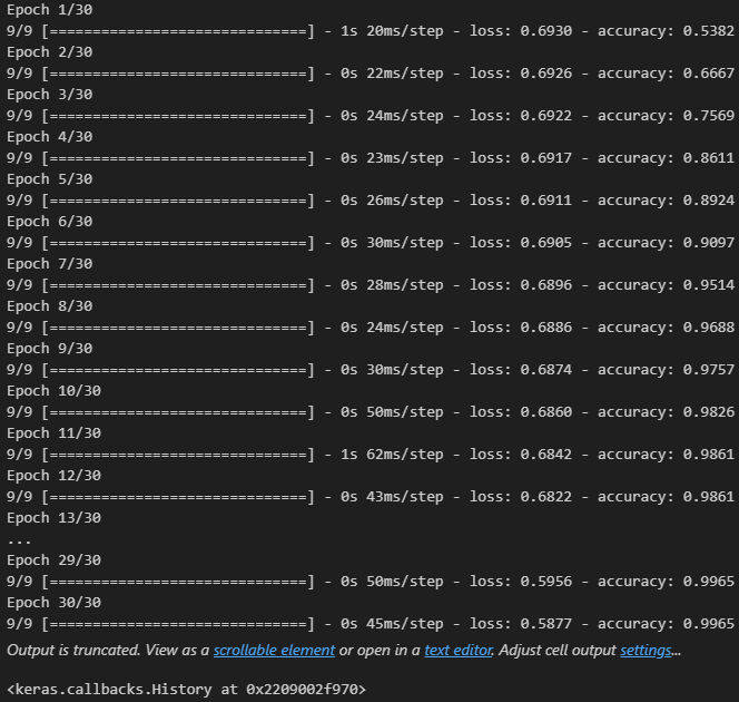
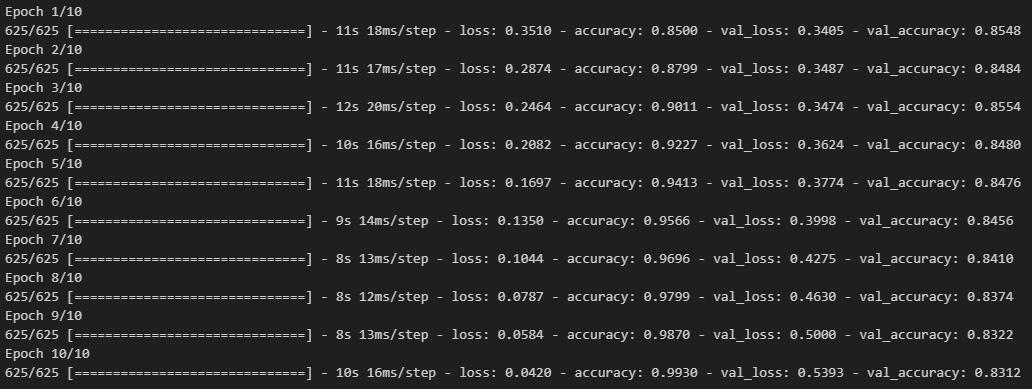
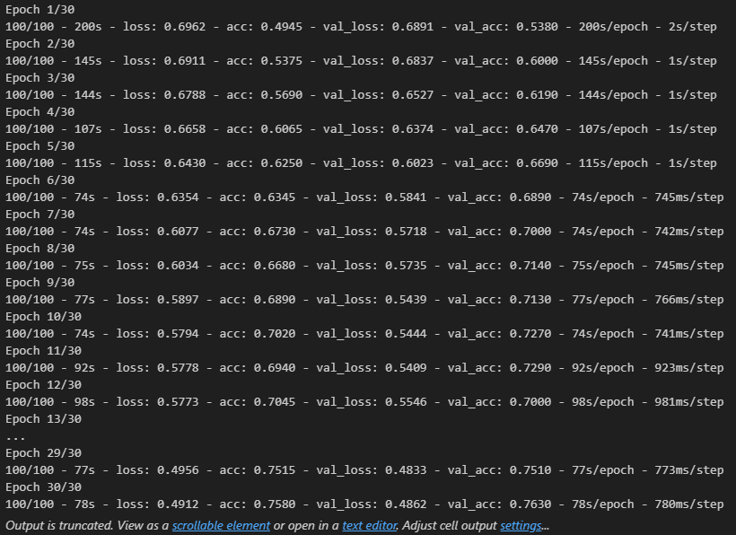
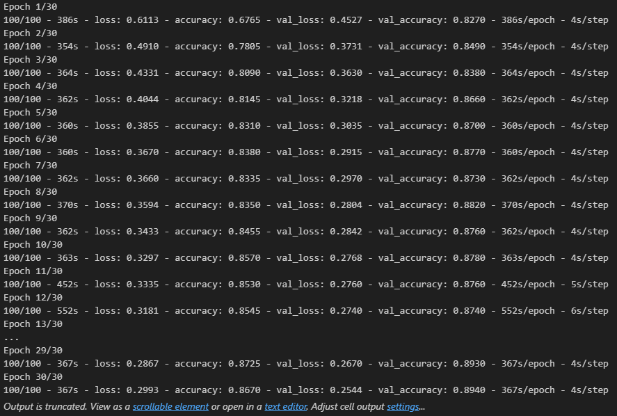
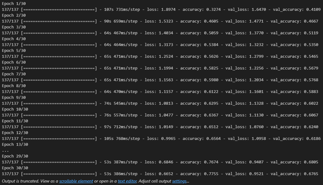
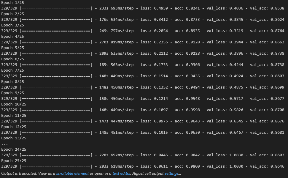
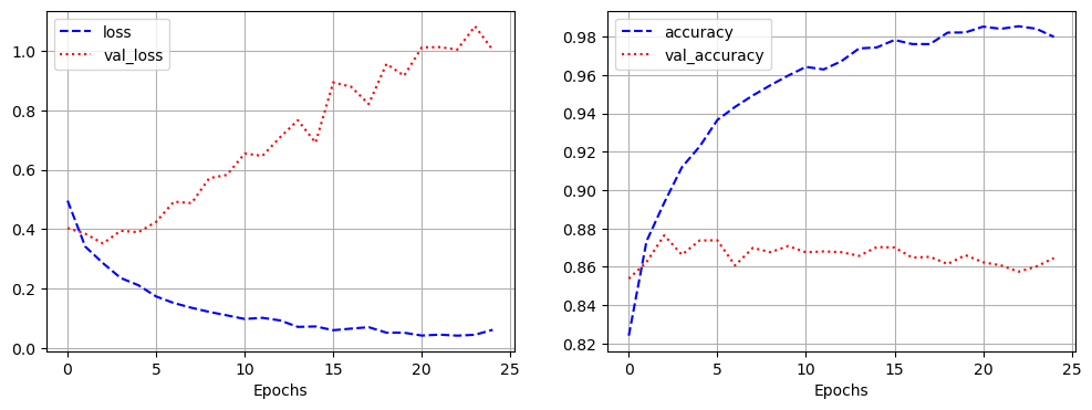
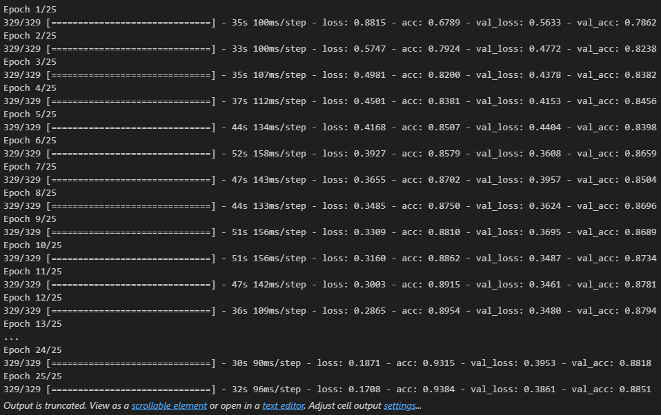
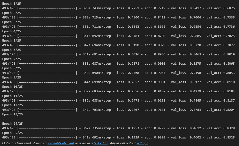
- 모델 학습
history = model.fit(pad_x_train, y_train,
                    epochs = 30,
                    batch_size = 128,
                    validation_split = 0.2)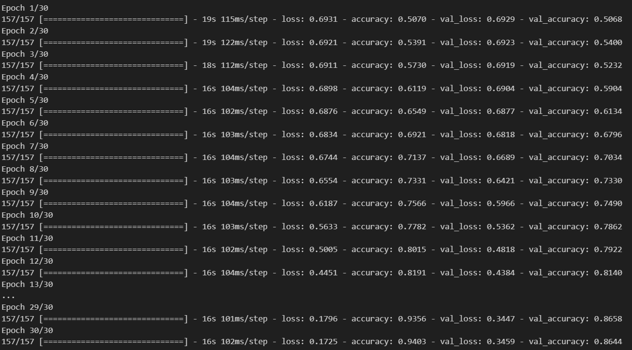
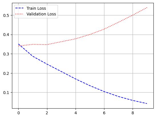
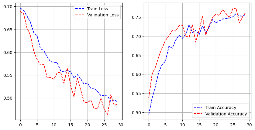
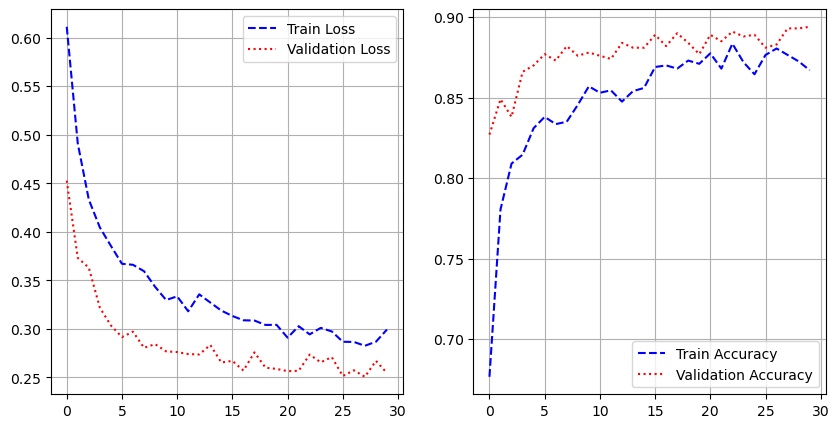
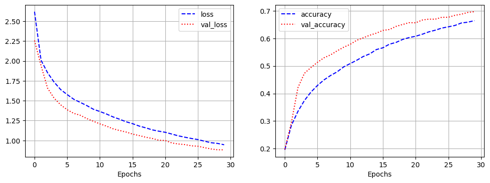
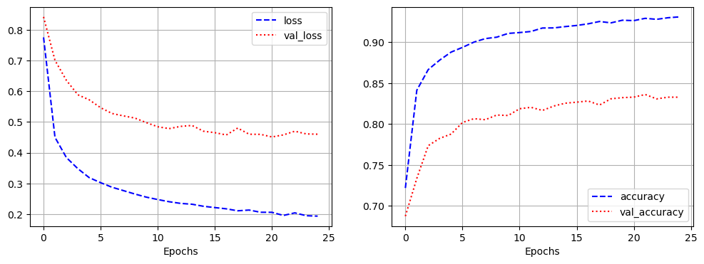
- 시각화
import matplotlib.pyplot as plt
loss = history.history['loss']
val_loss = history.history['val_loss']
acc = history.history['accuracy']
val_acc = history.history['val_accuracy']
epochs = range(1, len(loss) + 1)
plt.plot(epochs, loss, 'b--', label = 'train loss')
plt.plot(epochs, val_loss, 'r:', label = 'validation loss')
plt.grid()
plt.legend()
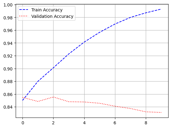
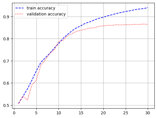
plt.figure()
plt.plot(epochs, acc, 'b--', label = 'train accuracy')
plt.plot(epochs, val_acc, 'r:', label = 'validation accuracy')
plt.grid()
plt.legend()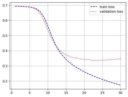
model.evaluate(pad_x_test, y_test)

# 출력 결과
loss: 0.3534 - accuracy: 0.8526
[0.35335206985473633, 0.8525999784469604]- 과적합이 일어났지만, 다른 optimizer 사용, 규제화를 걸어보는 등 다양하게 시도해볼 수 있음
'Python > Deep Learning' 카테고리의 다른 글
| [딥러닝-케라스] 케라스 텍스트 처리 및 임베딩(2) (0) | 2023.05.18 |
|---|---|
| [딥러닝-케라스] 케라스 텍스트 처리 및 임베딩(1) (0) | 2023.05.17 |
| [딥러닝-케라스] 케라스 전이학습 (1) | 2023.05.17 |
| [딥러닝-케라스] 케라스 CIFAR10 CNN 모델 (0) | 2023.05.16 |
| [딥러닝-케라스] 케라스 Fashion MNIST CNN 모델 (0) | 2023.05.14 |