import tensorflow as tf
from tensorflow.keras.layers import Conv2D
import matplotlib.pyplot as plt
import numpy as np
from sklearn.datasets import load_sample_image
china = load_sample_image('china.jpg') / 255.print(china.dtype)
print(china.shape)
# 출력 결과
float64
(427, 640, 3)
plt.imshow(china)
plt.show
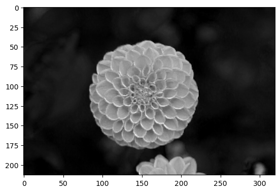
flower = load_sample_image('flower.jpg') / 255.print(flower.dtype)
print(flower.shape)
# 출력 결과
float64
(427, 640, 3)
plt.imshow(flower)
plt.show()
images = np.array([china, flower])
batch_size, height, width, channels = images.shape
print(images.shape)

# 출력 결과
(2, 427, 640, 3)
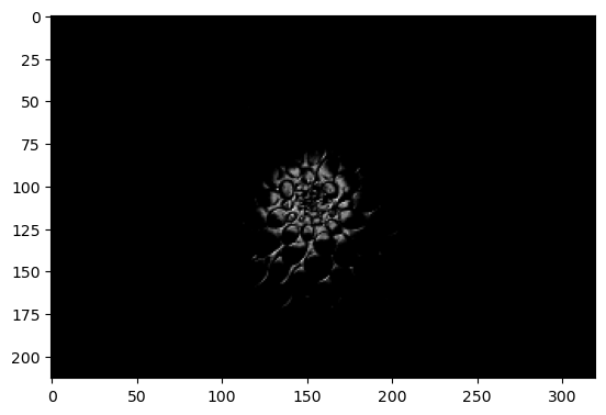
# 필터 적용
filters = np.zeros(shape = (7, 7, channels, 2), dtype = np.float32)
# 수직선 추가
filters[:, 3, :, 0] = 1# 수평선 추가
filters[3, :, :, 1] = 1print(filters.shape)
# 출력 결과
(7, 7, 3, 2)
# 텐서플로우로 conv2d 사용하는 방법
outputs = tf.nn.conv2d(images, filters, strides = 1, padding = 'SAME')
print(outputs.shape)
plt.imshow(outputs[0, :, :, 1], cmap = 'gray')
plt.show()

# 출력 결과
(2, 427, 640, 2)
from tensorflow.keras.layers import GlobalAvgPool2D

output = Conv2D(filters = 32, kernel_size=  3, strides = 1, padding = 'SAME', activation = 'relu')(flower)
output = GlobalAvgPool2D()(output)
output.shape

# 출력 결과
TensorShape([1, 32])
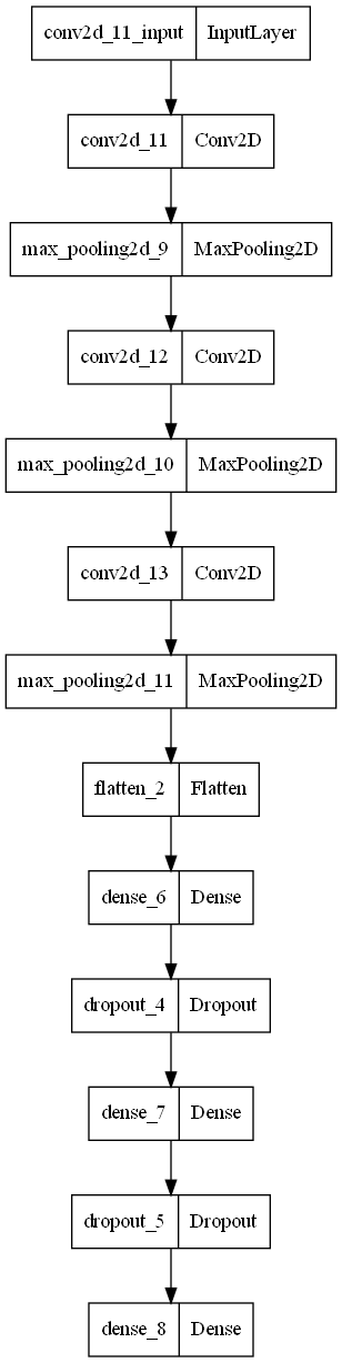
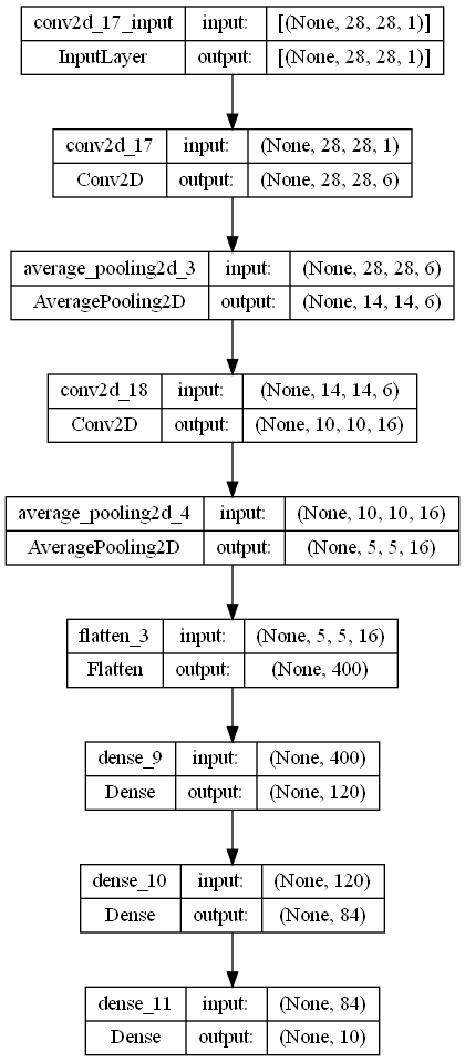
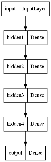
2. 예제로 보는 CNN 구조와 학습
● 일반적인 구조
- modules import
%load_ext tensorboard

import datetime
import numpy as np
import tensorflow as tf
import matplotlib.pyplot as plt

from tensorflow.keras import Model
from tensorflow.keras.models import Sequential
from tensorflow.keras.layers import Dense, Flatten, Conv2D, MaxPool2D, AvgPool2D, Dropout

from tensorflow.keras import datasets
from tensorflow.keras.utils import to_categorical, plot_model
- 데이터 로드 및 전처리
(x_train, y_train), (x_test, y_test) = datasets.fashion_mnist.load_data()
# 원본 데이터 형태print(x_train.shape)
print(y_train.shape)
print(x_test.shape)
print(y_test.shape)
# 출력 결과
(60000, 28, 28)
(60000,)
(10000, 28, 28)
(10000,)
# x 데이터에 축 하나씩 추가
x_train = x_train[:, :, :, np.newaxis]
x_test = x_test[:, :, :, np.newaxis]
print(x_train.shape)
print(x_test.shape)
# 출력 결과
(60000, 28, 28, 1)
(10000, 28, 28, 1)
# y 데이터 카테고리화
num_classes = 10
y_train = to_categorical(y_train, num_classes)
y_test = to_categorical(y_test, num_classes)
print(y_train.shape)
print(y_test.shape)
# 출력 결과print(y_train.shape)
print(y_test.shape)
# x 데이터 표준화
x_train = x_train.astype('float32')
x_test = x_test.astype('float32')
x_train /= 255.
x_test /= 255.
import datetime
import numpy as np
import tensorflow as tf
import matplotlib.pyplot as plt

from tensorflow.keras import Model
from tensorflow.keras.models import Sequential
from tensorflow.keras.layers import Dense, Flatten, Conv2D, MaxPool2D, AvgPool2D, Dropout

from tensorflow.keras import datasets
from tensorflow.keras.utils import to_categorical, plot_model

from sklearn.model_selection import train_test_split
import numpy as np
num_items = 20
num_list = np.arange(num_items)
num_list_dataset = tf.data.Dataset.from_tensor_slices(num_list)
num_list_dataset
# 출력 결과# shape은 아직 없는 상태
<TensorSliceDataset element_spec=TensorSpec(shape=(), dtype=tf.int32, name=None)>
output_types, output_shapes 인수로 출력 자료형과 크기를 지정해주어야 함
import itertools
# i는 1씩 증가하고 i의 개수만큼 1을 배열에 추가defgen():for i in itertools.count(1):
yield(i, [1] * i)
# 위에서 만든 generator# 출력 형식은 int64# 출력 형태는 TensorShape([])
dataset = tf.data.Dataset.from_generator(
gen,
(tf.int64, tf.int64),
(tf.TensorShape([]), tf.TensorShape([None]))
)
list(dataset.take(3).as_numpy_iterator())
# 출력 결과
[(1, array([1], dtype=int64)),
(2, array([1, 1], dtype=int64)),
(3, array([1, 1, 1], dtype=int64))]
# stop이 없이 위의 코드와 같이 gen을 돌리면 무한히 돌아감defgen(stop):for i in itertools.count(1):
if i < stop:
yield(i, [1] * i)
dataset = tf.data.Dataset.from_generator(
gen, args = [10],
output_types = (tf.int64, tf.int64),
output_shapes = (tf.TensorShape([]), tf.TensorShape([None]))
)
list(dataset.take(5).as_numpy_iterator())
# 출력 결과
[(1, array([1], dtype=int64)),
(2, array([1, 1], dtype=int64)),
(3, array([1, 1, 1], dtype=int64)),
(4, array([1, 1, 1, 1], dtype=int64)),
(5, array([1, 1, 1, 1, 1], dtype=int64))]
- batch, repeat
batch(): 배치 사이즈 크기
repeat(): 반복 횟수
# 배치사이즈 7, 3번 반복
dataset = num_list_dataset.repeat(3).batch(7)
for item in dataset:
print(item)
# 출력 결과# 배치 사이즈가 7이므로 7개씩 나뉨# 그렇게 3번 반복
tf.Tensor([0123456], shape=(7,), dtype=int32)
tf.Tensor([ 78910111213], shape=(7,), dtype=int32)
tf.Tensor([1415161718190], shape=(7,), dtype=int32)
tf.Tensor([1234567], shape=(7,), dtype=int32)
tf.Tensor([ 891011121314], shape=(7,), dtype=int32)
tf.Tensor([151617181901], shape=(7,), dtype=int32)
tf.Tensor([2345678], shape=(7,), dtype=int32)
tf.Tensor([ 9101112131415], shape=(7,), dtype=int32)
tf.Tensor([16171819], shape=(4,), dtype=int32)
# 뒤에 남는 수 없이 정확한 배치 사이즈로 나누어 떨어지도록 하고 싶으면# drop_remainder = True 옵션 설정
dataset = num_list_dataset.repeat(3).batch(7, drop_remainder = True)
for item in dataset:
print(item)
# 출력 결과# 마지막에 4개만 있던 데이터 사라짐
tf.Tensor([0123456], shape=(7,), dtype=int32)
tf.Tensor([ 78910111213], shape=(7,), dtype=int32)
tf.Tensor([1415161718190], shape=(7,), dtype=int32)
tf.Tensor([1234567], shape=(7,), dtype=int32)
tf.Tensor([ 891011121314], shape=(7,), dtype=int32)
tf.Tensor([151617181901], shape=(7,), dtype=int32)
tf.Tensor([2345678], shape=(7,), dtype=int32)
tf.Tensor([ 9101112131415], shape=(7,), dtype=int32)
- map, filter
전처리 단계레서 시행하여 원하지 않는 데이터를 거를 수 있음
tf.Tensor 자료형을 다룸
# map 함수 적용from tensorflow.data import Dataset
# [1, 2, 3, 4, 5]의 리스트
dataset = Dataset.range(1, 6)
# 리스트 각 값에 2씩 곱하는 과정을 map 함수로 적용
dataset = dataset.map(lambda x: x * 2)
list(dataset.as_numpy_iterator())
# 출력 결과
[2, 4, 6, 8, 10]
# as_numpy_iterator()형태로 출력하지 않고 그대로 출력하는 경우
dataset = Dataset.range(5)
result = dataset.map(lambda x: x + 1)
result
# 출력 결과
<MapDataset element_spec=TensorSpec(shape=(), dtype=tf.int64, name=None)>
# map 함수를 사용해 원하는 데이터만 전처리하여 가져올 수 있음
elements = [(1, 'one'), (2, 'two'), (3, 'three')]
dataset = Dataset.from_generator(lambda: elements, (tf.int32, tf.string))
result = dataset.map(lambda x_int, y_str: x_int)
list(result.as_numpy_iterator())

# 출력 결과
[1, 2, 3]
dataset = Dataset.range(3)
# 1. 기본적인 선언defg(x):return tf.constant(10.5), tf.constant(['One', 'Two', 'Three'])
result = dataset.map(g)
# 각 원소의 스펙 확인
result.element_spec
# 출력 결과
(TensorSpec(shape=(), dtype=tf.float32, name=None),
TensorSpec(shape=(3,), dtype=tf.string, name=None))
# 2. tf.constant로 텐서플로우 타입을 명시하지 않아도 기본적으로 적용됨defh(x):return10.5, ['One', 'Two', 'Three'], np.array([1., 2.], dtype = np.float64)
result = dataset.map(h)
result.element_spec
# 출력 결과
(TensorSpec(shape=(), dtype=tf.float32, name=None),
TensorSpec(shape=(3,), dtype=tf.string, name=None),
TensorSpec(shape=(2,), dtype=tf.float64, name=None))
# 3. 내부에 데이터 리스트 형태 추가defi(x):return (10.5, [12.5, 11.1]), "One", "Two"
result = dataset.map(i)
result.element_spec
# 출력 결과
((TensorSpec(shape=(), dtype=tf.float32, name=None),
TensorSpec(shape=(2,), dtype=tf.float32, name=None)),
TensorSpec(shape=(), dtype=tf.string, name=None),
TensorSpec(shape=(), dtype=tf.string, name=None))
# 1. 필터로 조건 지정
dataset = Dataset.from_tensor_slices([1, 2, 3])
dataset = dataset.filter(lambda x: x < 3)
list(dataset.as_numpy_iterator())
# 출력 결과
[1, 2]
# 2. 필터를 함수로 지정가능# 1이랑 같은 것만 필터링deffilter_fn(x):return tf.math.equal(x, 1)
dataset = dataset.filter(filter_fn)
list(dataset.as_numpy_iterator())
- shuffle, take
# 데이터 가져오기
dataset, info = tfds.load('imdb_reviews', with_info = True, as_supervised = True)

train_dataset = dataset['train']
# 5개로 구분하여 셔플하고, 2개를 가져오기
train_dataset = train_dataset.batch(5).shuffle(5).take(2)

for data in train_dataset:
    print(data)

# 출력 결과(영화 리뷰 데이터를 5개 가져와 섞은 뒤 그 중 2개를 출력한 것)
(<tf.Tensor: shape=(5,), dtype=string, numpy=
array([b'It was disgusting and painful. What a waste of a cast! I swear, the audience (1/2 full) laughed TWICE in 90 minutes. This is not a lie. Do not even rent it.<br /><br />Zeta Jones was just too mean to be believable.<br /><br />Cusack was OK. Just OK. I felt sorry for him (the actor) in case people remember this mess.<br /><br />Roberts was the same as she always is. Charming and sweet, but with no purpose. The "romance" with John was completely unbelievable.',
       b'This is a straight-to-video movie, so it should go without saying that it\'s not going to rival the first Lion King, but that said, this was downright good.<br /><br />My kids loved this, but that\'s a given, they love anything that\'s a cartoon. The big shock was that *I* liked it too, it was laugh out loud funny at some parts (even the fart jokes*), had lots of rather creative tie-ins with the first movie, and even some jokes that you had to be older to understand (but without being risqu\xc3\xa9 like in Shrek ["do you think he\'s compensating for something?"]).<br /><br />A special note on the fart jokes, I was surprised to find that none of the jokes were just toilet noises (in fact there were almost no noises/imagery at all, the references were actually rather subtle), they actually had a setup/punchline/etc, and were almost in good taste. I\'d like my kids to think that there\'s more to humor than going to the bathroom, and this movie is fine in those regards.<br /><br />Hmm what else? The music was so-so, not nearly as creative as in the first or second movie, but plenty of fun for the kids. No painfully corny moments, which was a blessing for me. A little action but nothing too scary (the Secret of NIMH gave my kids nightmares, not sure a G rating was appropriate for that one...)<br /><br />All in all I\'d say this is a great movie for kids of any age, one that\'s 100% safe to let them watch (I try not to be overly sensitive but I\'ve had to jump up and turn off the TV during a few movies that were less kid-appropriate than expected) - but you\'re safe to leave the room during this one. I\'d say stick around anyway though, you might find that you enjoy it too :)',
       b'Finally, Timon and Pumbaa in their own film...<br /><br />\'The Lion King 1 1/2: Hakuna Matata\' is an irreverent new take on a classic tale. Which classic tale, you ask? Why, \'The Lion King\' of course!<br /><br />Yep, if there\'s one thing that Disney is never short of, it\'s narcissism.<br /><br />But that doesn\'t mean that this isn\'t a good film. It\'s basically the events of \'The Lion King\' as told from Timon and Pumbaa\'s perspective. And it\'s because of this that you\'ll have to know the story of \'The Lion King\' by heart to see where they\'re coming from.<br /><br />Anyway, at one level I was watching this and thinking "Oh my god this is so lame..." and on another level I was having a ball. Much of the humour is predictable - I mean, when Pumbaa makes up two beds, a big one for himself and a small one for Timon, within the first nanosecond we all know that Timon is going to take the big one. But that doesn\'t stop it from being hilarious, which, IMO, is \'Hakuna Matata\' in a nutshell. It\'s not what happens, it\'s how.<br /><br />And a note of warning: there are also some fart jokes. Seriously, did you expect anything else in a film where Pumbaa takes centre stage? But as fart jokes go, these are especially good, and should satisfy even the most particular connoisseur.<br /><br />The returning voice talent is great. I\'m kinda surprised that some of the actors were willing to return, what with most of them only having two or three lines (if they\'re lucky). Whoopi Goldberg is particularly welcome.<br /><br />The music is also great. From \'Digga Tunnah\' at the start to \'That\'s all I need\', an adaption of \'Warthog Rhapsody\' (a song that was cut from \'The Lion King\' and is frankly much improved in this incarnation), the music leaves me with nothing to complain about whatsoever.<br /><br />In the end, Timon and Pumbaa are awesome characters, and while it may be argued that \'Hakuna Matata\' is simply an excuse to see them in various fun and assorted compromising situations then so be it. It\'s rare to find characters that you just want to spend time with.<br /><br />Am I starting to sound creepy?<br /><br />Either way, \'The Lion King 1 1/2\' is great if you\'ve seen \'The Lion King\' far too many times. Especially if you are right now thinking "Don\'t be silly, there\'s no such thing as seeing \'The Lion King\' too many times!"',
       b'Indian Directors have it tough, They have to compete with movies like "Laggan" where 11 henpecked,Castrated males defend their village and half of them are certifiable idiots. "Devdas", a hapless, fedar- festooned foreign return drinking to oblivion, with characters running in endless corridors oblivious to any one\'s feelings or sentiments-alas they live in an ornate squalor of red tapestry and pageantry. But to make a good movie, you have to tight-rope walk to appease the frontbenchers who are the quentessential gapers who are mesmerized with Split skirts and Dishum-Dishum fights preferably involving a nitwit "Bollywood" leading actor who is marginally handsome. So you can connect with a director who wants to tell a tale of Leonine village head who in own words "defending his Village" this is considered a violent movie or too masculine for a male audience. There are very few actors who can convey the anger and pathos like Nana Patekar (Narasimhan). Nana Patekar lets you in his courtyard and watch him beret and mock the Politician when his loyal admirers burst in laughter with every word of satire thrown at him, meanwhile his daughter is bathing his Grandson.This is as authentic a scene you can get in rural India. Nana Patekar is the essential actor who belongs to the old school of acting which is a disappearing breed in Hindi Films. The violence depicted is an intricate part of storytelling with Song&Dances thrown in for the gawkers without whom movies won\'t sell, a sad but true state of affairs. Faster this changes better for "Bollywood". All said and done this is one good Movie.',
       b"Nathan Detroit runs illegal craps games for high rollers in NYC, but the heat is on and he can't find a secure location. He bets chronic gambler Sky Masterson that Sky can't make a prim missionary, Sarah Brown, go out to dinner with him. Sky takes up the challenge, but both men have some surprises in store \xc2\x85<br /><br />This is one of those expensive fifties MGM musicals in splashy colour, with big sets, loud music, larger-than-life roles and performances to match; Broadway photographed for the big screen if you like that sort of thing, which I don't. My main problem with these type of movies is simply the music. I like all kinds of music, from Albinoni to ZZ Top, but Broadway show tunes in swing time with never-ending pah-pah-tah-dah trumpet flourishes at the end of every fourth bar aren't my cup of tea. This was written by the tag team of Frank Loesser, Mankiewicz, Jo Swerling and Abe Burrows (based on a couple of Damon Runyon stories), and while the plot is quite affable the songs are weak. Blaine's two numbers for example are identical, unnecessary, don't advance the plot and grate on the ears (and are also flagrantly misogynistic if that sort of thing bothers you). There are only two memorable tunes, Luck Be A Lady (sung by Brando, not Sinatra as you might expect) and Sit Down, You're Rockin' The Boat (nicely performed by Kaye) but you have to sit through two hours to get to them. The movie's trump card is a young Brando giving a thoughtful, laid-back performance; he also sings quite well and even dances a little, and is evenly matched with the always interesting Simmons. The sequence where the two of them escape to Havana for the night is a welcome respite from all the noise, bustle and vowel-murdering of Noo Yawk. Fans of musicals may dig this, but in my view a musical has to do something more than just film the stage show."],
      dtype=object)>, <tf.Tensor: shape=(5,), dtype=int64, numpy=array([0, 1, 1, 1, 0], dtype=int64)>)
(<tf.Tensor: shape=(5,), dtype=string, numpy=
array([b"This was an absolutely terrible movie. Don't be lured in by Christopher Walken or Michael Ironside. Both are great actors, but this must simply be their worst role in history. Even their great acting could not redeem this movie's ridiculous storyline. This movie is an early nineties US propaganda piece. The most pathetic scenes were those when the Columbian rebels were making their cases for revolutions. Maria Conchita Alonso appeared phony, and her pseudo-love affair with Walken was nothing but a pathetic emotional plug in a movie that was devoid of any real meaning. I am disappointed that there are movies like this, ruining actor's like Christopher Walken's good name. I could barely sit through it.",
       b'I have been known to fall asleep during films, but this is usually due to a combination of things including, really tired, being warm and comfortable on the sette and having just eaten a lot. However on this occasion I fell asleep because the film was rubbish. The plot development was constant. Constantly slow and boring. Things seemed to happen, but with no explanation of what was causing them or why. I admit, I may have missed part of the film, but i watched the majority of it and everything just seemed to happen of its own accord without any real concern for anything else. I cant recommend this film at all.',
       b'Mann photographs the Alberta Rocky Mountains in a superb fashion, and Jimmy Stewart and Walter Brennan give enjoyable performances as they always seem to do. <br /><br />But come on Hollywood - a Mountie telling the people of Dawson City, Yukon to elect themselves a marshal (yes a marshal!) and to enforce the law themselves, then gunfighters battling it out on the streets for control of the town? <br /><br />Nothing even remotely resembling that happened on the Canadian side of the border during the Klondike gold rush. Mr. Mann and company appear to have mistaken Dawson City for Deadwood, the Canadian North for the American Wild West.<br /><br />Canadian viewers be prepared for a Reefer Madness type of enjoyable howl with this ludicrous plot, or, to shake your head in disgust.',
       b'This is the kind of film for a snowy Sunday afternoon when the rest of the world can go ahead with its own business as you descend into a big arm-chair and mellow for a couple of hours. Wonderful performances from Cher and Nicolas Cage (as always) gently row the plot along. There are no rapids to cross, no dangerous waters, just a warm and witty paddle through New York life at its best. A family film in every sense and one that deserves the praise it received.',
       b'As others have mentioned, all the women that go nude in this film are mostly absolutely gorgeous. The plot very ably shows the hypocrisy of the female libido. When men are around they want to be pursued, but when no "men" are around, they become the pursuers of a 14 year old boy. And the boy becomes a man really fast (we should all be so lucky at this age!). He then gets up the courage to pursue his true love.'],
      dtype=object)>, <tf.Tensor: shape=(5,), dtype=int64, numpy=array([0, 0, 0, 1, 1], dtype=int64)>)
- get_next()
dataset = Dataset.range(2)
for element in dataset:
    print(element)

# 출력 결과
tf.Tensor(0, shape=(), dtype=int64)
tf.Tensor(1, shape=(), dtype=int64)
dataset = Dataset.range(2)
iterator = iter(dataset)
print(dataset)
# 다음 데이터에 접근print(iterator.get_next())
print(iterator.get_next())
# 출력 결과
<RangeDataset element_spec=TensorSpec(shape=(), dtype=tf.int64, name=None)>
tf.Tensor(0, shape=(), dtype=int64)
tf.Tensor(1, shape=(), dtype=int64)
a = np.random.randint(0, 10, size = (2, 3))
print(a)
dataset = Dataset.from_tensor_slices(a)
iterator = iter(dataset)
print(iterator.get_next())
print(iterator.get_next())
# 출력 결과# a의 원래 2행짜리 데이터에서 get_next()가 실행될 때마다 다음 행에 접근
[[072]
[614]]
tf.Tensor([072], shape=(3,), dtype=int32)
tf.Tensor([614], shape=(3,), dtype=int32)
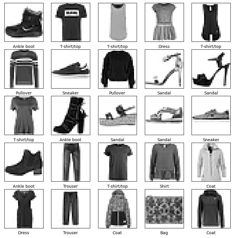
2. tf.dataset을 이용한 Fashion-MNIST 분류
- modules import
import matplotlib.pyplot as plt
import tensorflow as tf
from tensorflow.keras.layers import Dense, Input, Flatten, Dropout, Activation, BatchNormalization
from tensorflow.keras.models import Model
from tensorflow.keras.datasets.fashion_mnist import load_data
- 데이터 로드
(x_train, y_train), (x_test, y_test) = load_data()
# 데이터 형태 확인print(x_train.shape)
print(y_train.shape)
print(x_test.shape)
print(y_test.shape)
# 출력 결과
(60000, 28, 28)
(60000,)
(10000, 28, 28)
(10000,)
model.evaluate(x_test, y_test, batch_size = 100)

# 출력 결과
loss: 0.4427 - accuracy: 0.8464
[0.44270941615104675, 0.8464000225067139]
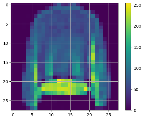
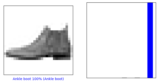
- 결과 확인
# 첫번째 테스트 데이터 결과
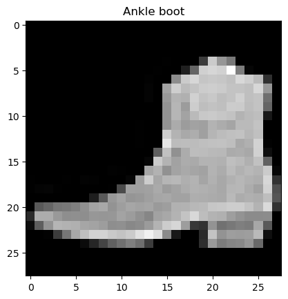
test_img = x_test[0, :, :]
plt.title(class_names[y_test[0]])
plt.imshow(test_img, cmap = 'gray')
plt.show()
pred = model.predict(test_img.reshape(1, 28, 28))
pred.shape
# 출력 결과
(1, 10)
pred
# 출력 결과
array([[8.9198991e-05, 3.5745958e-05, 7.4570953e-06, 1.5882608e-05,
8.0741156e-06, 3.3398017e-02, 4.0778108e-05, 1.1560775e-01,
7.1698561e-04, 8.5008013e-01]], dtype=float32)
# 가장 확률이 높은 것을 정답으로 출력
class_names[np.argmax(pred)]
# 출력 결과'Ankle boot'
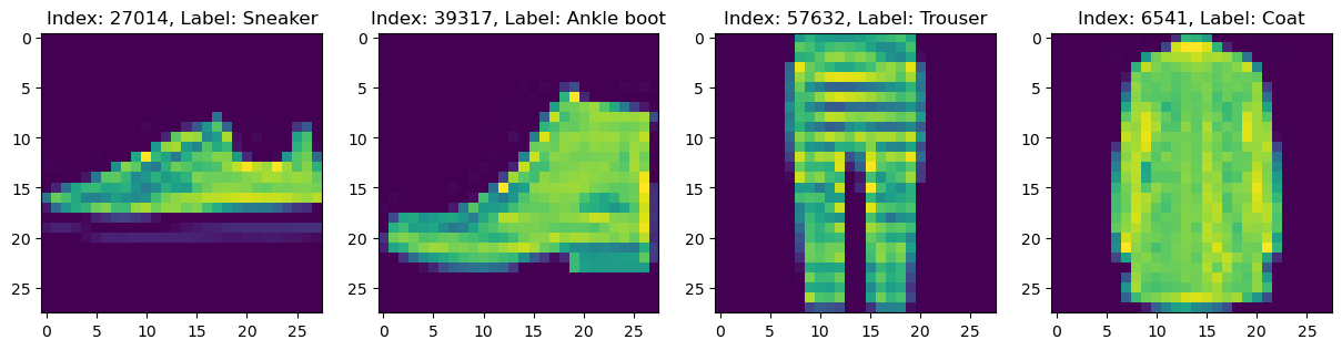
- Test Batch Dataset
test_batch = x_test[:32, :, :]
test_batch_y = y_test[:32]
print(test_batch.shape)

# 출력 결과
(32, 28, 28)
preds = model.predict(test_batch)
preds.shape

# 출력 결과
(32, 10)
from tensorflow.keras.optimizers import Adam

# beta_1과 beta_2에 지정한 값은 디폴트 값으로, 어느정도 가장 좋은 값이라고 증명된 값
optimizer = Adam(learning_rate = 0.001, beta_1 = 0.9, beta_2 = 0.999)
5. 배치 정규화
모델에 주입되는 샘플들을 균일하게 만드는 방법
학습 후 새로운 데이터에 잘 일반화 할 수 있도록 도와줌
데이터 전처리 단계에서 진행해도 되지만 정규화가 되어서 layer에 들어갔다는 보장이 없음
공공에는 거의 모든 분야에 대한 데이터가 존재하였고, 선택한 주제에 맞게 찾아 쓰면 아주 쉽게 데이터 수집을 할 수 있었습니다.
하지만 공공에 공개되는 데이터이다보니 개인정보의 문제도 있고 대용량이다보니 관리가 어려운 면이 있어 품질이 좋지는 못하다고 느꼈습니다. 또한, 매년 지속적으로 갱신되는 데이터는 매년 기준이나 입력자가 다르면 입력 내용이 통일되지 못해 방대한 전처리 과정이 필요한 경우도 있었습니다.
이런 경우, 빠른 시간 내에 데이터를 분석하기 어렵고 그 결과 또한 좋지 못한 경우도 있었습니다.
그래서 저는 데이터 품질이 데이터 분석 이전에 해결되어야 할 문제임을 확실하게 느낄 수 있었습니다. 데이터 분석가가 된다면 이런 공공 데이터를 사용할 때 이 품질을 어떻게 향상시켜 사용할 수 있을지, 사내 데이터를 사용한다면 품질을 어떻게 관리하고 사용해야하는지 알아두어야함을 깨달았습니다.
그래서 데이터 품질을 공부하기 위해 선택한 책이 '데이터 품질의 비밀'입니다.이 책은 O'REILLY의 데이터 품질에 관한 첫번째 책이며 한빛미디어의 임프린트인 디코딩에서 새로 출간된 책으로 데이터 품질에 대한 최신의 내용을 만나볼 수 있습니다.
책의 목차를 참고하여 이 책에서 배울수 있는 것은 다음과 같습니다.
데이터 품질이 중요한 이유
데이터 품질을 고려한 데이터 시스템 구축
데이터 수집·정제·변환·테스트 과정에서 데이터 품질 관리
데이터 파이프라인 모니터링 및 이상 탐지를 통한 품질 관리
데이터 신뢰성을 위한 아키텍처
대규모 데이터의 품질 문제 해결
엔드 투 엔트 데이터 계보 구축
데이터 품질 민주화
데이터 품질 관련 사례
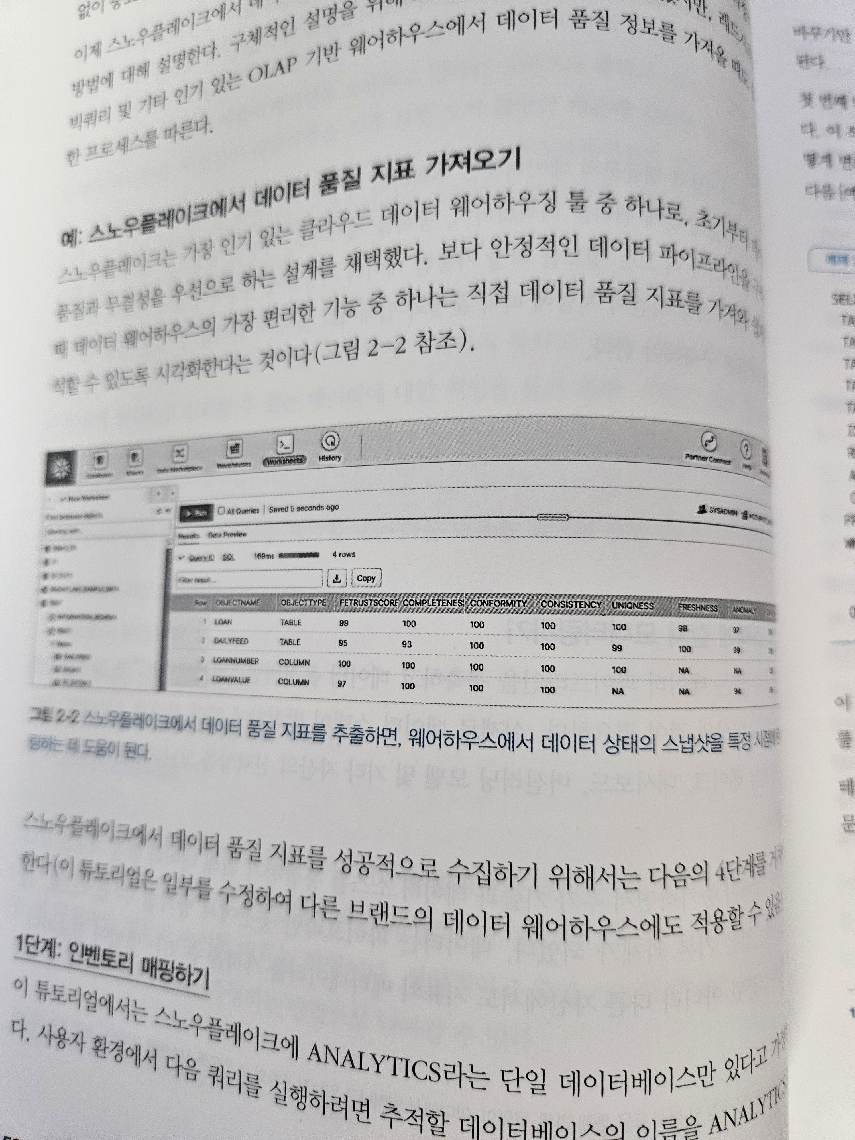
책에는 이해를 돕기위한 실제 툴의 사진도 삽입되어 있었고, SQL문으로 작성한 쿼리를 통해 더 유용한 쿼릴르 작성하는 방법을 구체적으로 학습할 수 있었습니다.
또한, 데이터 품질 관리를 위해 팀이 함께 수행해야할 업무를 구체적으로 알려주며 회사에도 공유하면 좋을 내용들이었습니다.
데이터 품질이 정말 중요하다고 느껴 공부하기 위해 서평 이벤트에 참여하여 해당 책을 받기는 했지만 정말 많은 도움이 되었던 것 같습니다. 데이터 품질에 관한 O'REILLY의 첫번째 책이라는 점에서 책장에 하나 쯤 있어도 좋겠다는 소장 욕구가 생기기도 하고 두고두고 데이터 품질을 관리하기 위해 읽을 수 있는 책인 것 같습니다.
import tensorflow as tf
from tensorflow.keras.datasets.fashion_mnist import load_data
from tensorflow.keras.models import Sequential, Model
from tensorflow.keras import models
from tensorflow.keras.layers import Dense, Input
from tensorflow.keras.optimizers import RMSprop
from tensorflow.keras.utils import plot_model

from sklearn.model_selection import train_test_split

import numpy as np
import matplotlib.pyplot as plt
# 정답의 집합
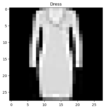
class_names = ['T-shirt/top', 'Trouser', 'Pullover', 'Dress', 'Coat',
'Sandal', 'Shirt', 'Sneaker', 'bag', 'Ankle boot']
# 첫번째 데이터의 정답 확인
class_names[y_train[0]]
# 출력 결과'Pullover'
pred_ys = model.predict(x_test)
print(pred_ys.shape)
np.set_printoptions(precision = 7)
print(pred_ys[0])
# 출력 결과# 정답 집합 10개 각각이 정답일 확률을 표시
(10000, 10)
[4.2854483e-211.0930411e-151.6151620e-173.9182383e-112.9266587e-153.3629590e-034.9878759e-171.0700015e-032.2493745e-139.9556702e-01]
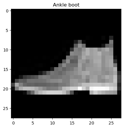
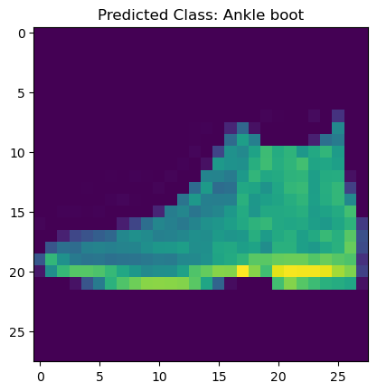
# 10개의 정답 집합 각각에 속할 확률 중 가장 높은 확률을 가진 값을 정답으로 채택하고 결과 확인
arg_pred_y = np.argmax(pred_ys, axis = 1)
plt.imshow(x_test[0].reshape(-1, 28))
plt.title('Predicted Class: {}'.format(class_names[arg_pred_y[0]]))
plt.show()
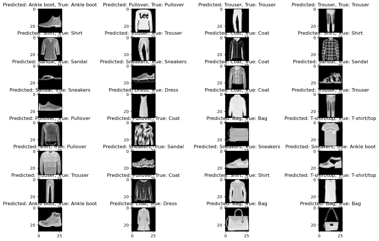
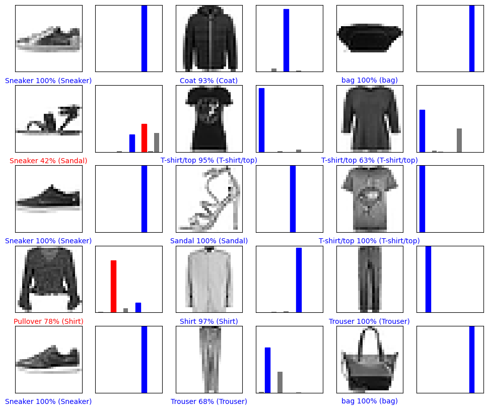
# 이미지 출력defplot_image(i, pred_ys, y_test, img):
pred_ys, y_test, img = pred_ys[i], y_test[i], img[i]
plt.grid(False)
plt.xticks([])
plt.yticks([])
plt.imshow(img, cmap = plt.cm.binary)
predicted_label = np.argmax(pred_ys)
if predicted_label == y_test:
color = 'blue'else:
color = 'red'
plt.xlabel("{} {:2.0f}% ({})".format(class_names[predicted_label],
100 * np.max(pred_ys),
class_names[y_test]),
color = color)
# 전체 정답 집합 중 해당 데이터를 정답으로 예측한 확률 표시defplot_value_array(i, pred_ys, true_label):
pred_ys, true_label = pred_ys[i], true_label[i]
plt.grid(False)
plt.xticks([])
plt.yticks([])
thisplot = plt.bar(range(10), pred_ys, color = '#777777')
plt.ylim([0, 1])
predicted_label = np.argmax(pred_ys)
thisplot[predicted_label].set_color('red')
thisplot[true_label].set_color('blue')
# 첫번째 데이터 정답 확인
i = 0
plt.figure(figsize = (8, 4))
plt.subplot(1, 2, 1)
plot_image(i, pred_ys, y_test, x_test.reshape(-1, 28, 28))
plt.subplot(1, 2, 2)
plot_value_array(i, pred_ys, y_test)
plt.show()
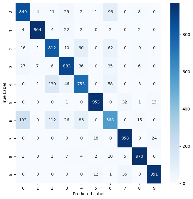
import pandas as pd
import seaborn as sns
import matplotlib.pyplot as plt

import tensorflow as tf
from tensorflow.keras.layers import Dense, Input
from tensorflow.keras.optimizers import RMSprop
from tensorflow.keras.models import Model
from tensorflow.keras.utils import get_file, plot_model
2. 데이터 로드
# 해당 주소의 데이터를 다운로드
dataset_path = get_file("auto-mpg.data", "http://archive.ics.uci.edu/ml/machine-learning-databases/auto-mpg/auto-mpg.data")
# 열 이름 지정
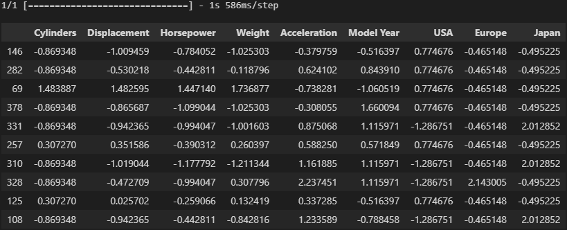
column_names = ['MPG', 'Cylinders', 'Displacement', 'Horsepower', 'Weight','Acceleration','Model Year', 'Origin']
# 지정된 열이름을 사용하여 데이터를 판다스 데이터프레임 형식으로 로드
raw_dataset = pd.read_csv(dataset_path, names = column_names,
na_values = '?', comment = '\t',
sep = ' ', skipinitialspace = True)
3. 데이터 확인
# raw data바로 사용하지 않고 copy()하여 사용
dataset = raw_dataset.copy()
dataset
4. 데이터 전처리
해당 데이터는 일부 데이터가 누락되어 있음
dataset.isna().sum()

# 출력 결과
MPG             0
Cylinders       0
Displacement    0
Horsepower      6
Weight          0
Acceleration    0
Model Year      0
Origin          0
dtype: int64
누락된 행 삭제
# Horsepower에 6개의 결측값이 있으므로 결측값 제거
dataset = dataset.dropna()
# train 데이터로 전체 데이터의 0.8을 추출# 전체 데이터에서 train 데이터를 drop시킨 나머지를 test 데이터로 지정
train_dataset = dataset.sample(frac = 0.8, random_state = 0)
test_dataset = dataset.drop(train_dataset.index)
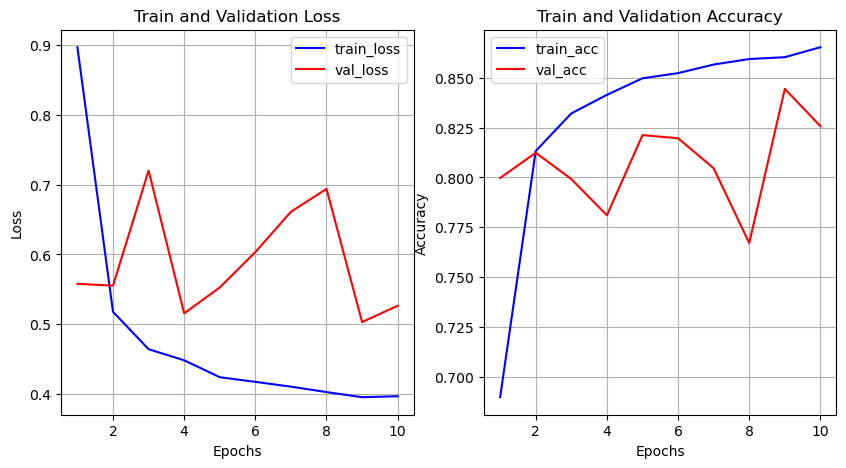
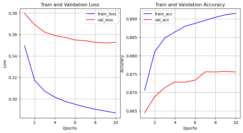
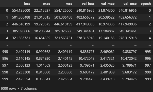
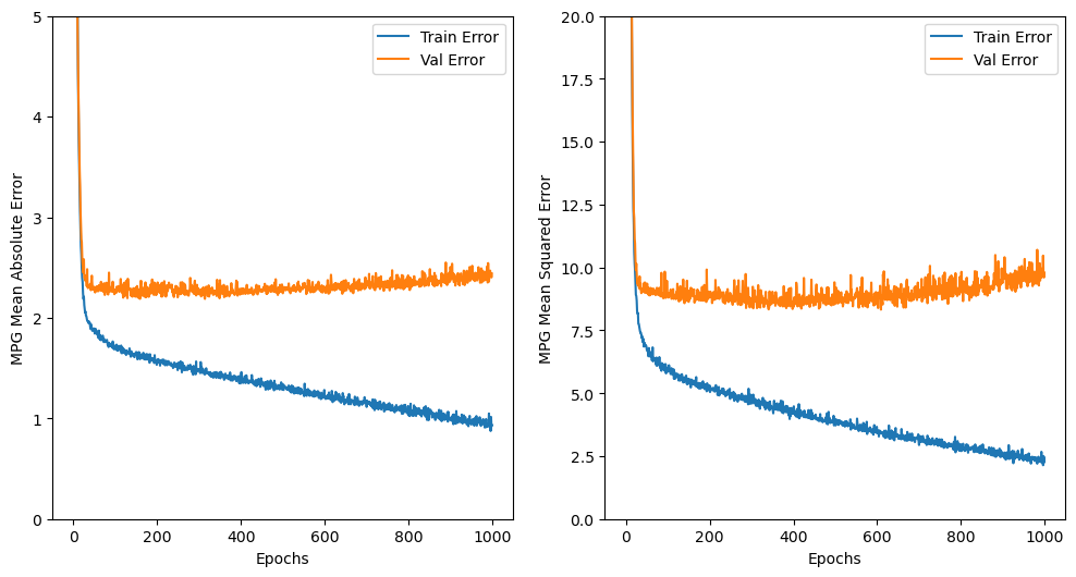
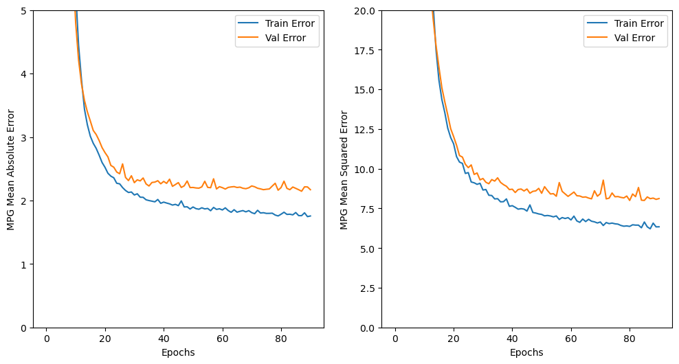
검증데이터의 오차(Val Error)값이 mae, mse 값 모두 일정 값 이하로 더이상 떨어지지 않음
학습을 더 진행해봤자 검증데이터의 오차가 줄어들지 않으면 의미가 없고 train 데이터의 오차만 줄어들어 둘 사이 간격이 벌어지면 오히려 모델이 train 데이터에 과대적합될 수 있음
9. EarlyStopping을 이용한 규제화
from tensorflow.keras.callbacks import EarlyStopping
model = build_model()
# 10번의 성능 향상을 보고 그 동안 성능 향상이 이뤄지지 않으면 stop
early_stop = EarlyStopping(monitor = 'val_loss', patience = 10)
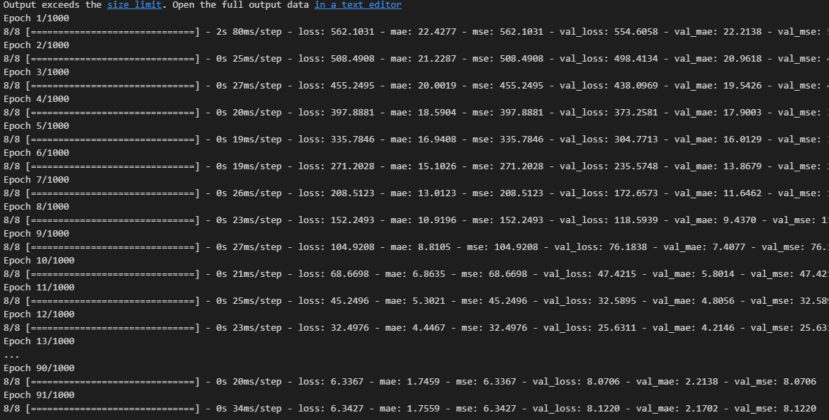
history = model.fit(normed_train_data, train_labels, epochs = epochs,
validation_split = 0.2, callbacks = [early_stop])
1000번 다 반복되지 않고 91번째에서 성능 향상이 없다고 판단되어 학습 중지
plot_history(history)
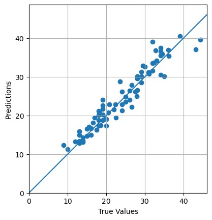
10. 모델 평가
# test 데이터를 모델에 넣어 나온 loss와 mae, mse 값 저장
loss, mae, mse = model.evaluate(normed_test_data, test_labels, verbose = 2)
print(mae)
# 출력 결과# 1.88정도의 mpg 오차내에서 예측3/3 - 0s - loss: 5.7125 - mae: 1.8831 - mse: 5.7125 - 61ms/epoch - 20ms/step
1.8831140995025635
import tensorflow as tf
from tensorflow.keras.datasets.boston_housing import load_data
from tensorflow.keras.layers import Dense
from tensorflow.keras.models import Sequential
from tensorflow.keras.optimizers import Adam
from tensorflow.keras.utils import plot_model

from sklearn.model_selection import train_test_split

import numpy as np
import matplotlib.pyplot as plt
# 가장 첫번째 train 데이터의 독립변수들print(x_train_full[0])
# 출력 결과
[2.8750e-022.8000e+011.5040e+010.0000e+004.6400e-016.2110e+002.8900e+013.6659e+004.0000e+002.7000e+021.8200e+013.9633e+026.2100e+00]
# 가장 첫번째 train 데이터의 종속변수print(y_train_full[0])
# 출력 결과25.0
3. 데이터 확인
print('학습 데이터: {}\t레이블: {}'.format(x_train_full.shape, y_train_full.shape))
print('테스트 데이터: {}\t레이블: {}'.format(x_test.shape, y_test.shape))
# 출력 결과
학습 데이터: (404, 13) 레이블: (404,)
테스트 데이터: (102, 13) 레이블: (102,)
from sklearn.model_selection import KFold
from tensorflow.keras.layers import Input
from tensorflow.keras.models import Model
tf.random.set_seed(111)
(x_train_full, y_train_full), (x_test, y_test) = load_data(path = 'boston_housing.npz',
                                                           test_split = 0.2,
                                                           seed = 111)
mean = np.mean(x_train_full, axis = 0)
std = np.std(x_train_full, axis = 0)
x_train_preprocessed = (x_train_full - mean) / std
x_test = (x_test - mean) / std
# 3개로 나누는 KFold 모델 생성
k = 3
kfold = KFold(n_splits = k, random_state = 111, shuffle = True)
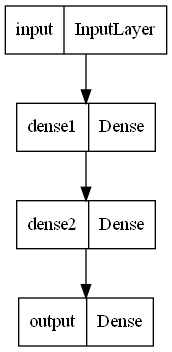
# 모델 생성defbuild_model():input = Input(shape = (13, ), name = 'input')
hidden1 = Dense(100, activation = 'relu', input_shape = (13, ), name = 'dense1')(input)
hidden2 = Dense(64, activation = 'relu', name = 'dense2')(hidden1)
hidden3 = Dense(32, activation = 'relu', name = 'dense3')(hidden2)
output = Dense(1, name = 'output')(hidden3)
model = Model(inputs = [input], outputs = [output])
model.compile(loss = 'mse',
optimizer = 'adam',
metrics = ['mae'])
return model
# mae값을 저장할 리스트
mae_list = []
# 각 fold마다 학습 진행for train_idx, val_idx in kfold.split(x_train):
x_train_fold, x_val_fold = x_train[train_idx], x_train[val_idx]
y_train_fold, y_val_fold = y_train_full[train_idx], y_train_full[val_idx]
model = build_model()
model.fit(x_train_fold, y_train_fold, epochs = 300,
validation_data = (x_val_fold, y_val_fold))
_, test_mae = model.evaluate(x_test, y_test)
mae_list.append(test_mae)
print(mae_list)
print(np.mean(mae_list))
# 출력 결과# 기준이 $1000이므로 $8000정도의 오차범위가 존재한다는 의미
[9.665495872497559, 8.393745422363281, 8.736763954162598]
8.932001749674479